3.1.3.3 - Supply and its determinants
Learn why sellers offer more output at a higher price, how changes in production conditions shift supply, and why a competitive firm's supply decision is connected to marginal cost.
Supply and price
A supply curve shows the quantity sellers are willing and able to offer at each price during a stated period, holding other influences constant. Supply is a planned flow, such as loaves per day. It is neither the stock sitting in a warehouse nor the quantity consumers want to buy.
In this illustrative bakery schedule, production costs and available ovens are unchanged:
| Price per loaf | Quantity supplied per day |
|---|---|
| £2 | 100 |
| £3 | 200 |
| £4 | 300 |
The quantity supplied increases from 100 to 300 as the loaf's own price rises. This is an extension of supply, a movement along the same curve. A fall in price causes a contraction along it. The term “increase in supply” is normally reserved for a shift of the whole curve.
To construct this graph on paper, put quantity per day on the horizontal axis and price per loaf on the vertical axis, select evenly spaced scales and plot each price–quantity pair. Join the points to show the relationship and label the curve S. The graph extends the schedule as an illustrative model; it does not prove that every bakery can expand indefinitely.
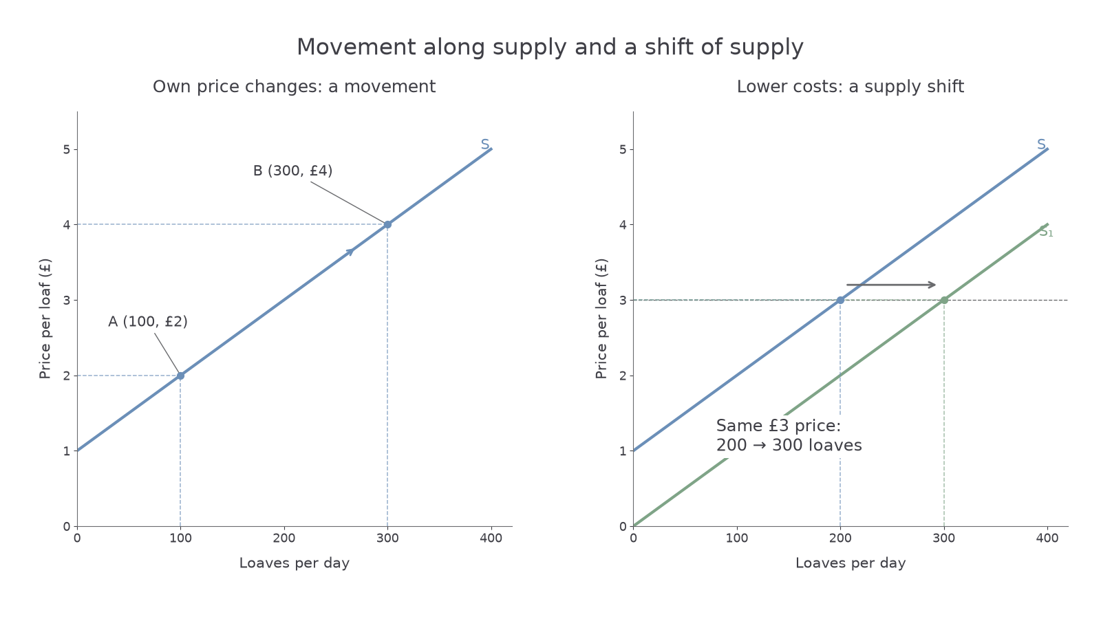
The left panel holds production conditions fixed: A is 100 loaves at £2 and B is 300 at £4. Read quantity by projecting down to the horizontal axis and price by projecting across to the vertical axis. The right panel compares quantities at an unchanged price and therefore shows a different event.
Profit incentives and additional output
A higher selling price makes additional production more rewarding when costs and other conditions are unchanged. At the original output, each unit earns more revenue, so total profit would be higher. Sellers therefore have an incentive to use overtime, operate another shift or bring less convenient resources into use.
The decision concerns the margin: compare the extra revenue from one more unit with its extra production cost. If an additional batch costs £70 and would sell for £60, producing it reduces profit. If its selling revenue rises to £80 while its cost stays £70, it adds £10 to profit and becomes worthwhile. This explains an upward-sloping supply curve rather than merely stating that price and quantity move together.
Expansion can raise the cost of the next unit: overtime is expensive, less suitable land must be used or a fixed machine becomes crowded. Progressively higher prices can make these increasingly costly units worth offering. The curve records that incentive under the model's conditions; it is not a claim that every price rise guarantees higher realised profit. An input-cost rise at the same time could remove the gain, and unsold output earns no sales revenue.
A producer also needs the ability to respond. A theatre with all seats sold cannot add seats tonight just because tickets become more valuable. Supply responsiveness is developed in the next lesson.
Changes in production conditions
A shift in supply occurs when sellers offer a different quantity at every given price because something other than that product's own price changes. A rightward shift means more is offered at each price; a leftward shift means less.
In the right panel above, S gives 200 loaves per day at £3. An improved oven reduces the cost of baking and moves supply to S₁, where 300 are offered at £3. The price has not caused this change. On the same axes, draw the new curve to the right and use a horizontal arrow between curves. A higher electricity bill would tend to shift supply left instead.
| Change, other things equal | Supply effect | Mechanism |
|---|---|---|
| Lower wages or raw-material prices | Right | Lower costs make additional units profitable at a given output price |
| Higher productivity or better technology | Right | Fewer inputs are needed per unit |
| A per-unit production tax | Left | Selling an extra unit now creates an extra tax cost |
| A per-unit production subsidy | Right | The producer receives support for each additional unit |
| More firms enter the market | Market supply right | More sellers offer output at each price |
| A crop disease or adverse weather | Agricultural supply left | Less output can be produced from available resources |
Expectations can matter: a seller able to store a commodity may withhold some current supply if a much higher future price is expected. That is a present supply shift, not a movement caused by the current price. Storage limits and spoilage can restrict this response.
When firms share inputs between products, a higher price for another product can divert resources away from this one. For example, more profitable wheat may reduce land available for barley, shifting barley supply left. Interrelated markets develop this link later.
Comparisons must hold the product's own price constant. If a survey reports more output sold alongside a higher price, it does not by itself establish a supply shift: demand may have increased, creating movement along unchanged supply.
Competitive supply and marginal cost
For a price-taking, profit-maximising firm, marginal cost is the cost of producing one additional unit, and the market price is the extra revenue from selling that unit. Under perfect competition, a firm can sell its relevant output at the given market price without changing that price.
If price exceeds marginal cost, an extra unit adds more revenue than cost, so the firm can increase profit by expanding. If marginal cost exceeds price, producing that extra unit reduces profit. On the relevant rising part of the marginal-cost curve, the chosen output is therefore where:
Suppose an illustrative firm faces marginal costs of £3, £4 and £5 for its 101st, 102nd and 103rd units. At a price of £4, the 101st adds £1 to profit, the 102nd adds zero at the margin, and the 103rd would reduce profit by £1. It expands through the £4 marginal unit rather than producing every unit simply because sales bring revenue.
This is the sense in which the competitive firm's supply curve is its marginal-cost curve. There is a qualification: in the short run, it is the rising portion above the minimum average variable cost at which operating is worthwhile. Below that threshold, shutting down avoids variable costs; it does not remove fixed costs already committed. At the threshold a firm can be indifferent between operating and shutting down. A fuller cost-curve treatment follows later in the course.
Market supply aggregates firms' quantities at each common price. It is not the marginal-cost curve of an entire industry treated as one monopolist. The price-taking argument cannot be transferred unchanged to a firm that must cut price on existing sales to sell extra output.