3.1.1.5 - Production possibility diagrams

The boundary of feasible production

A production possibility frontier shows the maximum combinations of two outputs attainable with given resources and technology over a stated period.

The production possibility frontier (PPF) is also called a production possibility curve. The model groups all output into two categories and holds the quantity and quality of resources and technology fixed. Points on the boundary assume those resources are used efficiently. It simplifies the real economy, but makes its physical production constraint visible.

The following economy is illustrative. Machines are measured in units per year on the horizontal axis; food in tonnes per year on the vertical axis. These are quantities of output, not prices or money values.

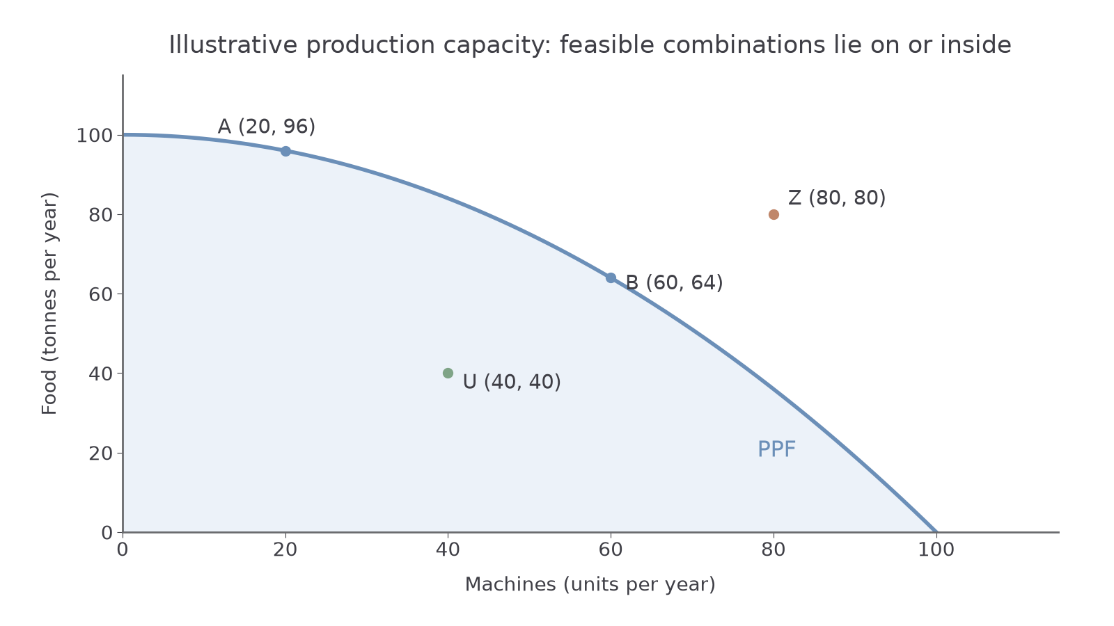
At A the economy produces 20 machines and 96 tonnes of food per year; at B it produces 60 machines and 64 tonnes. Both lie on the boundary. U, at 40 machines and 40 tonnes, lies inside: it is feasible, but the economy could produce more with its existing capacity. Z, at 80 machines and 80 tonnes, lies outside: that combination is currently unattainable under the stated resources and technology. “Unattainable” describes the current constraint, not what will remain impossible forever.

The intercepts show specialisation in one output: 100 tonnes of food and no machines, or 100 machines and no food. They do not mean the economy can produce both maxima together. The boundary is the set of feasible maximum combinations, not a target requiring one particular mix.

Drawing the representation

In your notebook, label two output axes and their units and period, choose readable scales, and plot the supplied maximum combinations. Join them with the frontier's indicated shape. Mark an interior and an exterior point and label the frontier. For this illustration, the boundary includes (0, 100), (20, 96), (40, 84), (60, 64), (80, 36) and (100, 0), with machines listed first. A smooth bowed curve through them is appropriate. If data specify constant trade-offs, use a straight line instead; do not add curvature by habit.

Notebook drawing develops the skill of representing the model. The marked text questions here assess what a supplied representation means; they do not verify an uploaded drawing.

Opportunity cost and the frontier's shape

Moving along the frontier reallocates resources between outputs, so gaining one output requires giving up another.

In the bowed-frontier illustration, moving from A to C increases machines from 20 to 40 but reduces food from 96 to 84 tonnes. The opportunity cost of the 20 extra machines is 12 tonnes of food. Per extra machine, this is:

Moving from C to B also gains 20 machines, but now food falls from 84 to 64: 20 tonnes are forgone, or 1 tonne per machine. Moving from B to D gains another 20 machines and forgoes 28 tonnes, or 1.4 tonnes per machine. Keep total output forgone separate from opportunity cost per extra unit. Use the loss of the alternative output divided by the gain in the chosen output, not the final output totals.

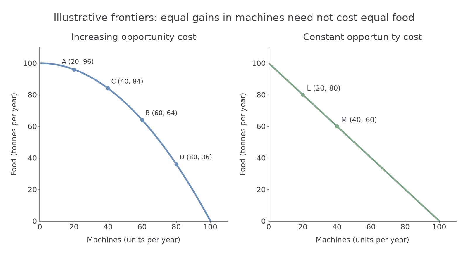
The bowed frontier reflects increasing opportunity cost. Resources are not equally suited to both activities. Initially, switching resources especially suitable for machine production sacrifices relatively little food. Further expansion requires transferring resources better suited to food, so each equal gain in machines costs more food. The curve becomes steeper as machines increase. Its slope's magnitude represents the trade-off; a negative slope does not mean the economic cost is a negative quantity of food.

The straight-line comparison describes a different illustrative economy. Moving from L (20 machines, 80 tonnes of food) to M (40, 60) costs 20 tonnes for 20 machines: 1 tonne per machine. Every equal increase in machines has that same trade-off. A straight line assumes constant opportunity cost, as where resources are equally adaptable between the two activities. Curvature is an economic assumption, not decoration.

Unused resources and changing capacity

An increase in actual output can come from using existing capacity better or from increasing the capacity itself.

An interior point such as U can reflect unemployed workers, idle machines or inefficient use of inputs. Moving towards the existing frontier brings more resources into effective use or reduces inefficiency. From U (40 machines, 40 tonnes of food), the illustration can reach (40, 84): more food with no loss of machines. The boundary has not shifted. This shows why a trade-off is not inevitable for every increase in actual output: unused capacity may allow both outputs to rise.

Once on the frontier, producing more of both outputs requires a change in what is possible. Growth in productive capacity shifts the frontier outwards. More or better capital, a larger or better-skilled workforce, or improved technology can enable greater output from the productive system. In the left panel, the maximum possible outputs of both machines and food rise from 100 to 120. A previously exterior combination may become feasible.

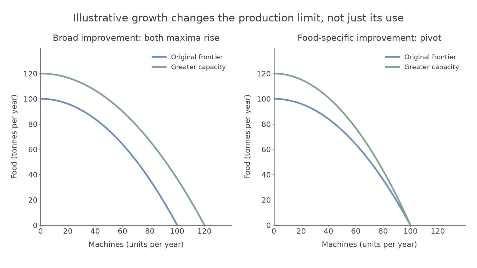
A shift need not be even. The right panel shows an improvement specifically in food production: its maximum rises to 120 tonnes, while the maximum number of machines remains 100. The frontier pivots outwards. Do not claim that every technological improvement increases every output by the same proportion.

Capacity growth is a potential increase, not proof that all new capacity is already used. If resources remain idle, actual production can still be inside the new frontier. Conversely, actual production can grow during a recovery without an outward shift: the economy is using existing capacity more fully. Keep a change in actual output, a movement between efficient output mixes and a change in the boundary distinct.

The connection can also work over time. In this model, some machines are productive capital. Producing more of them today may require less current food on the frontier, but the capital can help expand future capacity if it is useful and maintained. Sacrificing present consumption does not guarantee growth: inappropriate investment or untrained workers may prevent the expected gains. Damage to productive resources, such as destruction of equipment or a loss of usable farmland, can instead shift the frontier inwards.

Productive and allocative efficiency

Using resources efficiently and choosing the most desirable output mix are different questions.

In the PPF model, productive efficiency means producing a combination where more of one output cannot be obtained without reducing the other, given resources and technology. Every point on the frontier meets that condition. At A or B, there is no unused productive potential within the model. A point inside does not: the same resources can achieve more output. Employing everyone is not sufficient by itself if inputs are used inefficiently.

Allocative efficiency concerns the mix of outputs that best satisfies society's needs and wants. An efficient factory can make something that people value less than a feasible alternative. Similarly, a frontier point can be productively efficient while allocating too many resources to machines relative to food, or vice versa, given society's preferences.

The shape of the frontier supplies information about feasibility and trade-offs. It does not supply information about how much society values each output. The fact that A and B are both on the frontier therefore establishes productive efficiency at both, but cannot establish that both are allocatively efficient. We need evidence about preferences and benefits relative to the alternatives forgone to judge the mix. Different people may disagree about the appropriate priorities and distribution, linking this question to value judgements.

Reallocating from B towards A produces more food and fewer machines. It may improve the allocation if society values the additional food more than the machines sacrificed. It does not expand the frontier or increase productive efficiency: both endpoints are already on the boundary. If preferences change while resources and technology are unchanged, the preferred point can change without any shift in productive capacity.

Quick recap

A frontier separates feasible combinations from currently unattainable ones. Movement along it reveals opportunity cost; movement towards it can use idle capacity; an outward shift increases capacity. Boundary points are productively efficient, while allocative efficiency also depends on the value of the output mix.