3.1.3.5 - Equilibrium and changing market prices
Learn how demand and supply determine a market-clearing price, why shortages and surpluses create pressure for adjustment, and how to explain new equilibria while checking the model's assumptions.
Market equilibrium
Equilibrium is a position with no tendency to change within the model. In a competitive product market, it occurs at the price where quantity demanded equals quantity supplied. Buyers' and sellers' plans are compatible: the market clears without excess demand or excess supply.
This illustrative weekly meal market has the following plans:
| Price per meal | Quantity demanded, thousands/week | Quantity supplied, thousands/week |
|---|---|---|
| £4 | 160 | 80 |
| £6 | 120 | 120 |
| £8 | 80 | 160 |
The equilibrium price is £6 and equilibrium quantity is 120,000 meals per week. That quantity is not the sum of demand and supply: the same meals are bought and sold. It is planned demand and supply that are equal, not necessarily every person's desired consumption. Someone unable or unwilling to pay £6 may still want a meal.
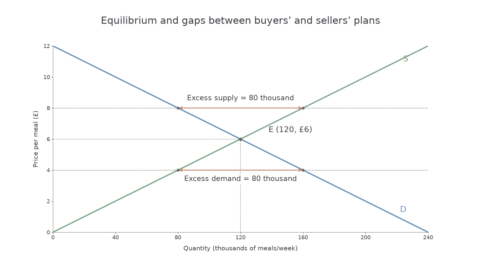
To construct the graph on paper, put quantity per week on the horizontal axis and price per meal on the vertical axis. Plot the schedule points, join each relationship and label D and S. Mark their intersection E, then project horizontally to £6 and vertically to 120. The graph's linear continuation is an illustrative assumption, not a measurement of every price.
Equilibrium is neither a claim that the outcome is fair nor proof of social efficiency. It describes consistency of market plans given the curves; income, environmental damage or other concerns require further models.
Shortages, surpluses and price adjustment
Disequilibrium means buyers' and sellers' plans do not match at the current price. A shortage is excess demand; a surplus is excess supply.
At £4 in the meal market, buyers demand 160,000 while sellers offer 80,000, so excess demand is:
Buyers compete for limited meals, and sellers can raise their prices without losing all customers. As price rises, quantity demanded contracts along D and quantity supplied extends along S. Both responses reduce the shortage until they meet at £6. The shortage itself has not shifted either curve.
At £8, sellers offer 160,000 and buyers demand 80,000, leaving 80,000 excess supply. Unsold output or accumulated stocks encourage sellers to cut prices. Lower prices extend demand and contract supply along the existing curves, reducing the surplus.
These are pressures for adjustment, not a guarantee of instant clearing. Sellers may be slow to alter prices; contracts, regulation or a fixed posted price may prevent adjustment. A shortage can instead appear as queues, waiting lists or rationing. Actual purchases can also be less than planned quantity supplied when goods remain unsold. Distinguish the curve's offer from completed transactions.
Changes in demand or supply
A new equilibrium arises when a non-price determinant shifts a curve and price then adjusts along the other curve. Start from a known equilibrium, identify the exogenous change and explain the temporary gap at the old price before moving to the new intersection.
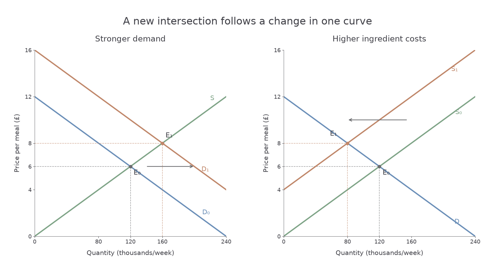
In the left panel, stronger preferences for delivered meals shift demand from D₀ to D₁. At the old £6 price, buyers now want more than 120,000 meals, creating excess demand. Price rises, encouraging movement up S and reducing quantity demanded relative to what buyers wanted at £6 on D₁. The new equilibrium E₁ is £8 and 160,000 meals. Demand shifts; supply extends along its unchanged curve.
In the right panel, higher ingredient costs shift supply from S₀ to S₁. At £6 sellers offer fewer meals than buyers demand, so a shortage puts upward pressure on price. Price rises until E₁ at £8 and 80,000 meals. The higher price contracts demand along D. The supply reduction and the induced contraction of demand are different steps in the same explanation.
The reverse changes follow the same logic: a demand decrease lowers equilibrium price and quantity; a supply increase lowers price and raises quantity, given conventional slopes. To draw a change, retain the original curves and equilibrium, label the shifted curve with a new subscript, then mark the new intersection and axis projections. Arrows should identify the shift between curves, not falsely shift the curve that only has a movement along it.
The mechanism transfers across markets. A frost affecting vegetables is a supply shock; a successful campaign encouraging train travel is a demand shock. Decide what changes before predicting price. An observed price rise alone cannot distinguish stronger demand from weaker supply: both can raise price, but their quantity implications differ.
When both curves change
If demand and supply change together, one outcome can be predictable while another depends on the relative changes. Do not force an exact new price or quantity from directions alone.
Suppose demand for bicycles rises and improved production technology also increases supply. The demand shift tends to raise price and quantity, while the supply shift tends to lower price and raise quantity. Both raise quantity, so quantity increases under the ordinary model. The price effects conflict: price could rise, fall or stay unchanged depending on the relative shifts and curve shapes.
If demand increases while supply decreases, both put upward pressure on price. Quantity is uncertain because stronger demand tends to raise it while weaker supply tends to lower it. If both demand and supply decrease, quantity falls but price is uncertain. These statements compare equilibria, not the order in which actual firms adjust.
For a numerical illustration, let original bicycle demand and supply be equal at £100 and 1,000 units. If the new curves still intersect at £100 but at 1,300 units, technology has offset the demand increase's price pressure exactly. A rightward demand shift does not necessarily raise the observed equilibrium price when other conditions change too.
Applying the model and checking assumptions
The basic demand-and-supply model isolates a market under conditions that make its predictions useful. It treats a defined product and period, holds non-investigated influences constant, assumes buyers and sellers respond to incentives, and normally allows prices to adjust. Competitive sellers take the market price rather than choosing a price through strategic market power. The curves represent planned behaviour under these conditions.
The price pressure from a supply loss is useful for analysing a crop shortage or a shipping disruption. Yet the predicted outcome depends on responsiveness and institutions. A perishable crop cannot be expanded overnight; warehouse stocks may soften a temporary disruption. A regulated price can leave a shortage rather than rising to the intersection. A sole seller may have strategic pricing decisions that the basic competitive model does not capture.
Consider an illustrative rental market. More students arriving shifts demand for rooms right. With a fixed number of available rooms in the immediate period, rents face upward pressure and quantity may respond little. If legal restrictions prevent rent increases, waiting lists and search costs can replace some price adjustment. Over time, converting buildings may increase supply, but planning rules and building costs can constrain that response. The model supplies a conditional chain, not a guarantee that every observed rental change has this cause.
Evidence helps choose the explanation. Higher prices and lower quantities are consistent with a supply decrease; higher prices and higher quantities are consistent with a demand increase, provided the other curve and measurement conditions are stable. Neither pattern alone proves causation in a market experiencing several shocks. Ask whether input costs, income, tastes, competing products, stocks or policy changed, and whether the data cover comparable products and periods.