3.1.3.2 - Price elasticity of demand
Learn to calculate and interpret consumers' responsiveness to price, explain what makes demand elastic or inelastic, and use the result to reason about total revenue.
Percentage change and its base
A percentage change compares a change with the original value, making differently sized markets comparable.
Percentage change
In original illustrative data, a ticket price rises from £10 to £12. The £2 increase is . Quantity demanded falls from 500 to 450 tickets per week: . Keep the negative sign for a fall and use the original quantity, not 450, as the base. Reversing the changes produces different percentages because the original values differ: £12 to £10 is a fall of approximately 16.7%, not 20%.
A percentage-point change compares two percentages directly. If a survey's proportion of consumers willing to switch brands rises from 20% to 25%, it rises by 5 percentage points. Its percentage increase is . Five and 25 answer different questions.
Separate a level from its growth rate. A price rising 10% this year after rising 20% last year is still increasing; its rate of increase has slowed by 10 percentage points. If it was £100 before both years, it becomes £120 then £132. A lower positive growth rate does not mean a lower price. These distinctions prevent a responsiveness calculation from using a change in a rate where it needs a change in the actual price or quantity.
Calculating and interpreting PED
Price elasticity of demand measures how much quantity demanded responds proportionately to a change in the product's own price, other things equal.
Price elasticity of demand
For the ticket example, . A 1% price rise is associated with approximately a 0.5% fall in quantity demanded around these conditions. PED has no units: it is a ratio of percentages, not tickets per pound. The negative sign reflects the usual opposite directions of price and quantity along a downward-sloping demand curve.
Use the absolute value to classify responsiveness, while retaining the signed answer in calculations. is more elastic than , even though it is numerically smaller on a number line.
| Absolute PED | Interpretation |
|---|---|
| Perfectly inelastic: quantity does not respond to price. The curve is vertical. | |
| Between 0 and 1 | Price inelastic: quantity changes proportionately less than price. |
| Unit elastic: equal proportionate responsiveness. | |
| Greater than 1 | Price elastic: quantity changes proportionately more than price. |
| Approaches infinity | Perfectly elastic: an arbitrarily small price rise from the given price loses demand. The idealised curve is horizontal. |
If a café's price falls 5% and quantity rises 15%, PED is , so demand is elastic. Do not reverse the fraction or infer elasticity from a large absolute quantity change alone. A rise of 100 units has a different meaning from an original 200 units than from an original 20,000.
These calculations estimate responsiveness over the supplied change using original-value percentage bases. Treat an estimate as conditional on the product, starting price, consumer group and period. If advertising also changes, the observed quantity response cannot be attributed solely to own price.
What determines responsiveness
Consumers respond strongly to a price change when they can and want to adjust their purchases.
Availability and closeness of substitutes are central. If several equivalent cafés are nearby, a price rise at one café makes switching easy. Demand for that café's coffee may be elastic. Demand for coffee as a whole can be less elastic because changing café does not reduce purchases across the whole coffee market. Define the market before comparing estimates.
Necessity and habits affect willingness to reduce consumption. A necessary journey to work is harder to give up than an optional outing. Habit or strong brand attachment can reduce switching, but no good is automatically perfectly inelastic merely because it is called necessary. Consumers may still change quantities or find alternatives.
The proportion of income spent affects the incentive to adjust. A price rise for an item taking a large share of a household budget creates more pressure to compare alternatives than a similar percentage rise for a tiny purchase. This is a tendency, conditional on substitutes and need, rather than a universal ranking.
Time affects ability to adjust. Immediately after a fuel price rise, a commuter may still drive because they own a car and live far from work. Over several years they could move, share journeys or use a more efficient vehicle. Demand may become more elastic as such alternatives become feasible. A short-run estimate therefore need not describe the longer run.
These factors interact. Strong loyalty can make demand for a differentiated brand relatively inelastic despite nearby competitors; easy comparison and weak loyalty can produce the opposite. Explain the route from the named factor to consumers' willingness or ability to change quantity, then to the proportional response.
Elasticity is not the slope
A demand curve's slope compares changes in price and quantity, while elasticity compares their percentage changes.
Changing pounds to pence makes a graph's numerical slope change even though consumers behave identically. PED does not change with that conversion because each percentage is unchanged. With comparable axes and the same starting price–quantity point, a flatter demand curve indicates greater local price responsiveness. Without those conditions, judging elasticity from appearance alone can mislead.
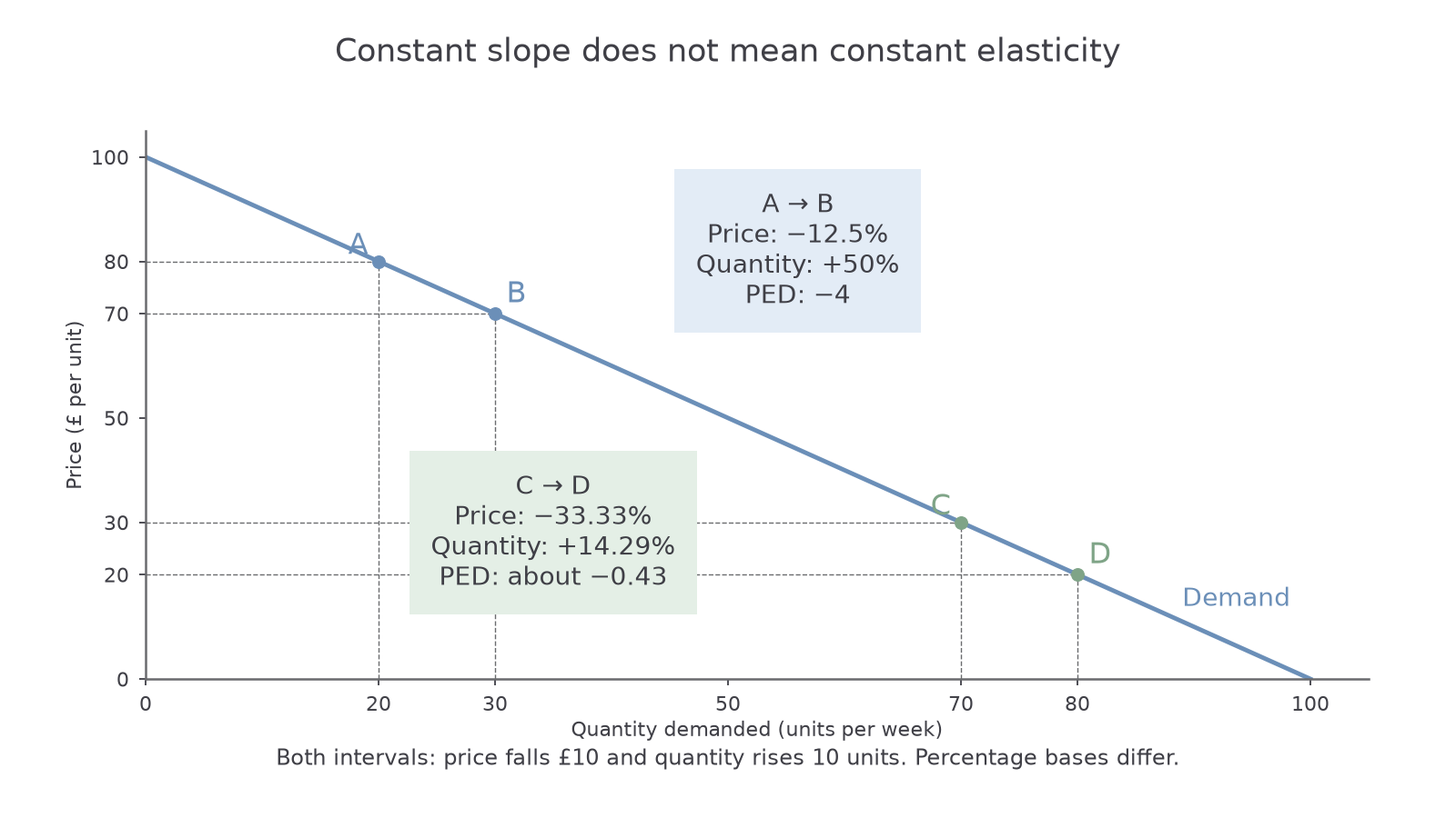
The diagram uses original illustrative data on one straight line. From A to B, price falls £80 to £70 and quantity rises 20 to 30 units per week. Quantity increases 50% while price falls 12.5%, so PED is . From C to D, price falls £30 to £20 and quantity rises 70 to 80. Quantity increases approximately 14.29% while price falls approximately 33.33%, so PED is about .
Both movements add 10 units after a £10 price fall. The slopes are identical, but the starting bases differ: ten units is a large proportion of 20 and a smaller proportion of 70. The upper interval is elastic; the lower interval is inelastic. A straight downward-sloping demand curve therefore need not have constant elasticity. Neither estimate says that demand shifted: each describes movement along the same curve.
To sketch the supplied relationship, label price and quantity axes, plot the stated coordinates and draw one straight line through them. Label the intervals rather than using a flatter line to represent the second calculation. The text assessment tests the interpretation, not performance of the drawing.
PED and total revenue
Total revenue depends on both the price received for each unit and the number of units sold.
Total revenue
Consumers' total expenditure on the product equals sellers' total revenue for those transactions. On a price–quantity graph it is the rectangle from the origin to the purchase point: height is price and width is quantity. In the following original examples all planned units are sold and other demand influences stay unchanged.
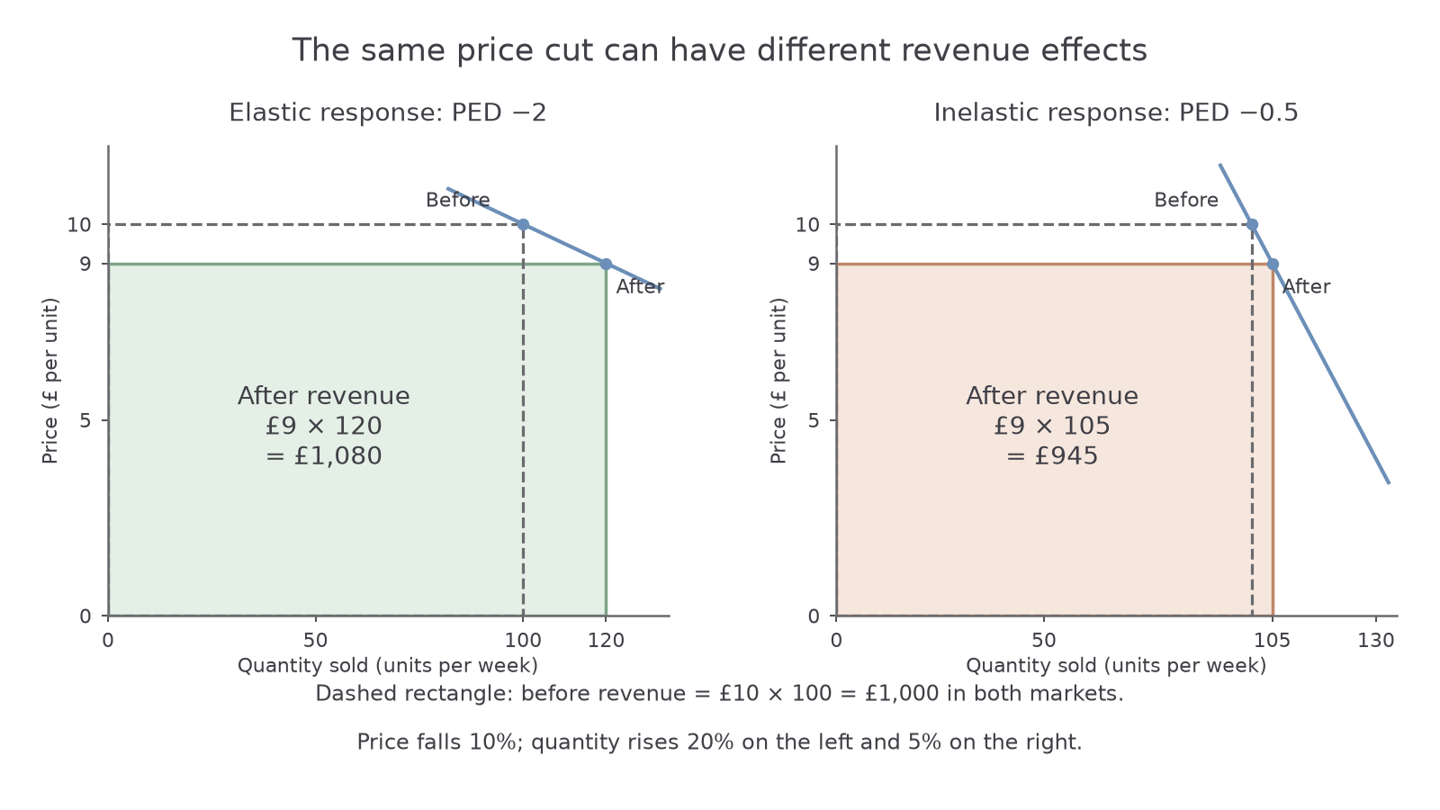
Both sellers cut price from £10 to £9 and initially sell 100 units per week. In the elastic case, quantity rises 20% to 120; PED is . Revenue rises from £1,000 to £1,080 because the extra quantity more than offsets the lower price per unit. In the inelastic case, quantity rises 5% to 105; PED is . Revenue falls to £945 because the extra sales are insufficient to offset the lower price.
For small changes along a stable curve, a price cut raises total revenue when demand is elastic and lowers it when demand is inelastic; a price rise reverses those directions. At unit elasticity, the two proportionate effects balance locally. A curve with unit elasticity throughout has constant total expenditure.
For a finite change, calculate at both points to establish the exact revenue effect. An original-base estimate of PED equal to is not an exact guarantee of unchanged revenue: a 10% price rise and a 10% quantity fall multiply revenue by . This does not overturn the local unit-elastic relationship; it shows why a finite estimate and an exact expenditure calculation must be distinguished.
A pricing decision also needs the goal and conditions. Extra revenue is not necessarily extra profit: supplying more units can increase costs. A venue with fixed seat capacity cannot sell unlimited extra tickets after a price cut. Competitors may react, and longer-run switching may differ from the estimate. PED helps predict the revenue mechanism; it does not alone establish the profit-maximising price.
Quick Recap
Use original values as the percentage-change bases, divide quantity's percentage change by price's, and retain its sign. Classify PED using its absolute size. Explain responsiveness through alternatives, need, budget share and time. Use exact price times quantity for finite revenue changes and keep revenue distinct from profit.