3.1.3.2 - Income and cross elasticities of demand
Learn how changes in income and other products' prices shift demand, calculate their elasticities, and use their signs and sizes to identify normal and inferior goods, substitutes and complements.
Calculating income elasticity
Income elasticity of demand measures how quantity demanded responds proportionately to a change in consumers' income, holding the product's own price and other influences constant.
Income elasticity of demand
Use the same original-value method for each percentage: . In an original illustrative household, monthly income rises from £2,000 to £2,200: a 10% increase. Restaurant visits rise from 4 to 5 per month: a 25% increase. Therefore . Around these conditions, a 1% income rise produces approximately a 2.5% rise in visits. YED has no units, even though the income is measured in pounds and visits per month.
Do not substitute the restaurant's price change into the denominator: that would be PED. Nor should you put income's percentage change in the numerator. If income instead falls 10% and visits fall 25%, YED remains positive because . A positive elasticity describes the same direction of response, rather than only an increase.
Maintain the distinction between income's level and growth rate. Income can still rise when its growth slows. If the growth rate falls from 6% to 4%, that is a fall of 2 percentage points in the rate; it is not a 2% fall in income. The YED denominator needs the percentage change in the income level relevant to purchasing power. An estimate based on money incomes during changing inflation needs care because higher money income may not mean greater real purchasing power.
Normal and inferior goods
The sign of YED identifies the direction of the income response; its size tells you how responsive the quantity is.
A normal good has positive YED: higher income raises demand, and lower income reduces it, other things equal. A normal good with is income inelastic, often described as a necessity. Quantity increases less proportionately than income. A normal good with is income elastic, often described as a luxury. Quantity increases more proportionately. At , it increases in the same proportion.
An inferior good has negative YED: as income rises, consumers switch away towards preferred alternatives. Inferior does not mean unsafe or badly made. A budget meal can be nutritious yet inferior for a household that buys more restaurant meals when its income rises. At YED zero, quantity has no income response over the conditions considered.
These classifications depend on the consumer group, initial income and product definition. As very low incomes rise, households may increase purchases of basic food substantially; at higher incomes extra spending can move to other goods. Preferences and the availability of alternatives also affect the response. A bus journey might be normal for one group but inferior for another able to afford a preferred way to travel. Necessity and luxury are economic descriptions of responsiveness, rather than moral judgements.
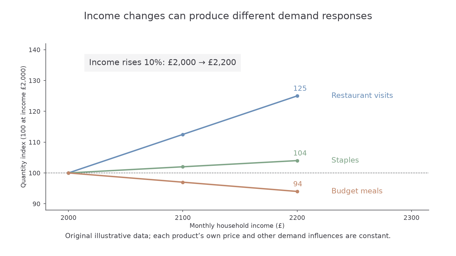
The graph holds own prices constant and compares changes from one base. Income rises from £2,000 to £2,200, or 10%. Restaurant quantity rises 100 to 125 on a quantity index, giving YED ; staples rise 100 to 104, giving ; budget meals fall 100 to 94, giving . The common quantity index makes proportional responses visible without adding unlike products. The upward and downward responses concern income on the horizontal axis; this is not a price–quantity demand curve.
Calculating cross elasticity
Cross elasticity of demand measures the response of demand for one product to a price change in a different product.
Cross elasticity of demand
Name A and B before calculating. In original illustrative data, the price of tea, B, rises from £2 to £2.20 per pack: . At an unchanged coffee price, demand for coffee, A, rises from 400 to 420 packs per week: . Coffee's XED with respect to tea's price is . Tea and coffee behave as substitutes in these conditions.
For a second case, the price of a games console, B, falls from £400 to £360, or . Demand for compatible games, A, rises from 1,000 to 1,200 per month, or , while game prices remain unchanged. Games' XED with respect to console price is : the opposite signs indicate complements.
Keep the denominator's direction. A complement's price increase may reduce demand for A, giving a negative numerator and positive denominator; its price decrease may increase demand for A, giving a positive numerator and negative denominator. Both produce negative XED.
This differs from PED. A change in coffee's own price moves along coffee's demand curve. A change in tea's price shifts coffee's demand curve because tea's price was held constant when that curve was drawn. XED gives the size and direction of the demand response at the unchanged own price. The two cross elasticities need not be equal: coffee's response to tea's price does not automatically tell you tea's response to coffee's price.
Substitutes, complements and closeness
XED's sign identifies the relationship between goods, while its magnitude indicates the strength of the measured cross-price response.
| XED | Interpretation, other things equal |
|---|---|
| Positive | Substitutes: a price rise for B increases demand for A as buyers switch towards it. |
| Negative | Complements: a price rise for B reduces demand for A because using them together becomes less attractive or affordable. |
| Zero or close to zero | No measured cross-price response, or a weak one, in the market and period considered. |
An XED of implies a larger proportional substitution response than to the same percentage rise in B's price. An XED of indicates a larger complementary response than . Do not call a substitute because its absolute value is small: sign and size answer different questions.
Closeness and range of alternatives matter. Two nearly identical drinks may be stronger substitutes than a drink and a distant alternative. Brand loyalty, switching costs and lack of information can weaken substitution. If there are many other alternatives, a price rise for B can spread switching across them rather than strongly increasing A alone.
For complements, the importance of joint use matters. A product that can only work with one specific refill may be tightly linked to it. An accessory used with many different products may have a weaker response to the price of any one. The response also depends on existing ownership: a household already owning a console may keep buying games despite a higher price for new consoles.
Time can strengthen a response as consumers discover substitutes or replace equipment. It can also alter the relationship through new technology and changing preferences. XED is therefore evidence about a defined pair of products in stated conditions. A near-zero estimate does not prove two goods have no conceivable connection.
Using demand elasticities
Elasticities convert a stated change in an influence into a conditional prediction for demand.
For small changes, rearrange the relevant formula:
Suppose a retailer's estimated YED is and household incomes are expected to rise 4%. Demand is predicted to rise approximately , holding its own price and other influences constant. If it initially sells 1,000 units per month, the estimate is 1,060 units. A luxury seller can therefore face a pronounced fall in demand when incomes fall; a seller of an inferior good could experience the opposite.
Alternatively, if A's XED with respect to B is and B's price rises 5%, predicted demand for A changes by . At 2,000 initial units that is 1,920. A supplier of complements may need to plan for lower sales when using the related product becomes more expensive.
Choose the formula from the cause, rather than from a product label. Own price requires PED, income requires YED, and another product's price requires XED. If own price is unchanged and all planned units are sold, a demand change alters the seller's revenue in the same proportion as quantity. This revenue statement does not establish profit because costs also matter.
When several influences change, an estimate for one influence does not isolate their combined effect. More income might raise demand for A while a complement's higher price reduces it. Estimates may vary by income group and over time, and observed income–quantity correlation may reflect another change such as product quality. Use the responsiveness to explain a mechanism, identify the held-constant assumptions, and judge whether the original estimate is relevant before making a business prediction. Tax incidence, labour demand and exchange-rate transmission build on these methods in later lessons.
Quick Recap
YED uses income in the denominator; XED uses another product's price. Retain signs to distinguish normal from inferior goods and substitutes from complements, then use magnitudes to interpret responsiveness. Both describe demand shifts at an unchanged own price, and predictions depend on the stated market, period and held-constant influences.