3.1.5.4 - Monopolistic competition

Differentiation and firm demand

Monopolistic competition combines many independent sellers, differentiated products and relatively easy entry and exit. Each firm supplies a small fraction of the market but has some control over its own price because its offer is not identical to rivals' offers. A café's menu, location and atmosphere can matter to buyers; nearby cafés remain close substitutes.

The individual firm's demand/average-revenue curve therefore slopes downward. Raising price loses some customers, while reducing price attracts others. It is usually more elastic when close substitutes are plentiful. Because the firm must reduce price to sell more units, marginal revenue is below average revenue: the extra unit adds revenue but the lower price also applies to earlier units in a uniform-price model.

The word “monopolistic” refers to limited power over a differentiated offer. The firm is not a pure monopolist over the broad market: many competing offers and entry constrain it. Many firms alone do not imply perfect competition either, since identical products and price-taking are absent. The strength of differentiation, geographical competition and entry conditions determine how useful this model is for a real market.

Short-run output, price and profit

A profit-maximising differentiated firm chooses output where rising MC crosses MR, then reads its price from demand/AR. It does not choose the MC–AR intersection and does not charge the MR value.

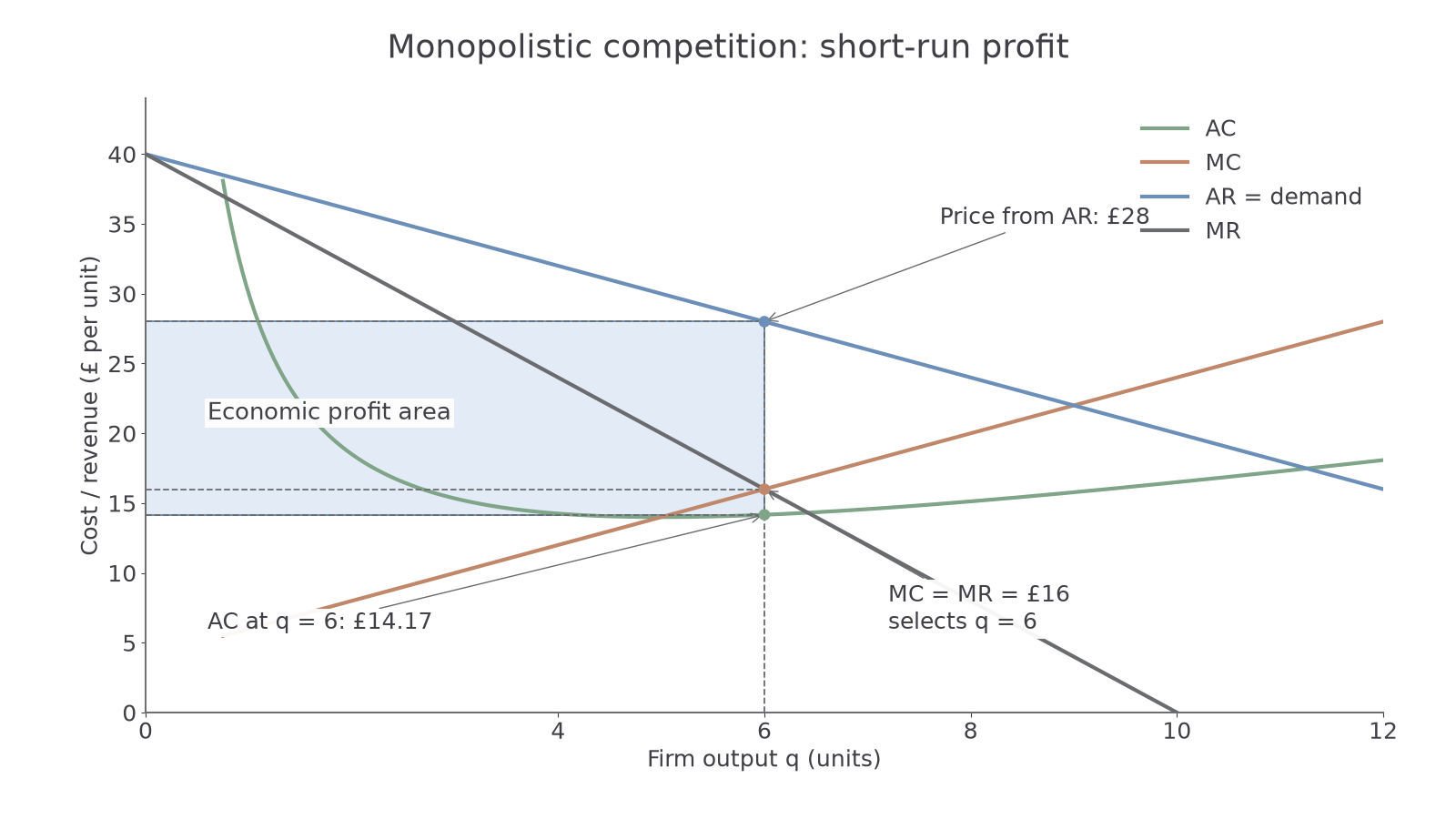
The original illustrative firm has demand $AR=40-2q$, marginal revenue $MR=40-4q$, and marginal cost $MC=4+2q$, all in pounds per unit. At q=6, MC=MR=£16; buyers pay £28 from AR. Its total economic cost is $TC=25+4q+q^2$, giving £85. Revenue is $6\times28=£168$, so economic profit is £83. Average cost is total cost divided by output: $AC=85/6$, approximately £14.17. The rectangle between price and AC over 6 units represents that profit. Normal profit is already in economic cost.

A firm can instead have a short-run loss if demand is too weak to cover AC at its best output. The market model does not guarantee profit. As in other firm models, short-run shutdown depends on whether revenue covers avoidable variable costs, while long-run survival requires full economic cost to be covered.

To draw the notebook model, label output and cost/revenue per unit. Add downward-sloping AR and a lower MR curve, coherent AC and MC, and mark the rising MC=MR intersection. Project vertically to AR for price and to AC for cost per unit; project horizontally to the vertical axis. Profit is the P−AC rectangle, not the distance between AR and MR. Text questions here assess reading and reasoning from a supplied graph; they do not prove drawing performance.

Entry and long-run excess capacity

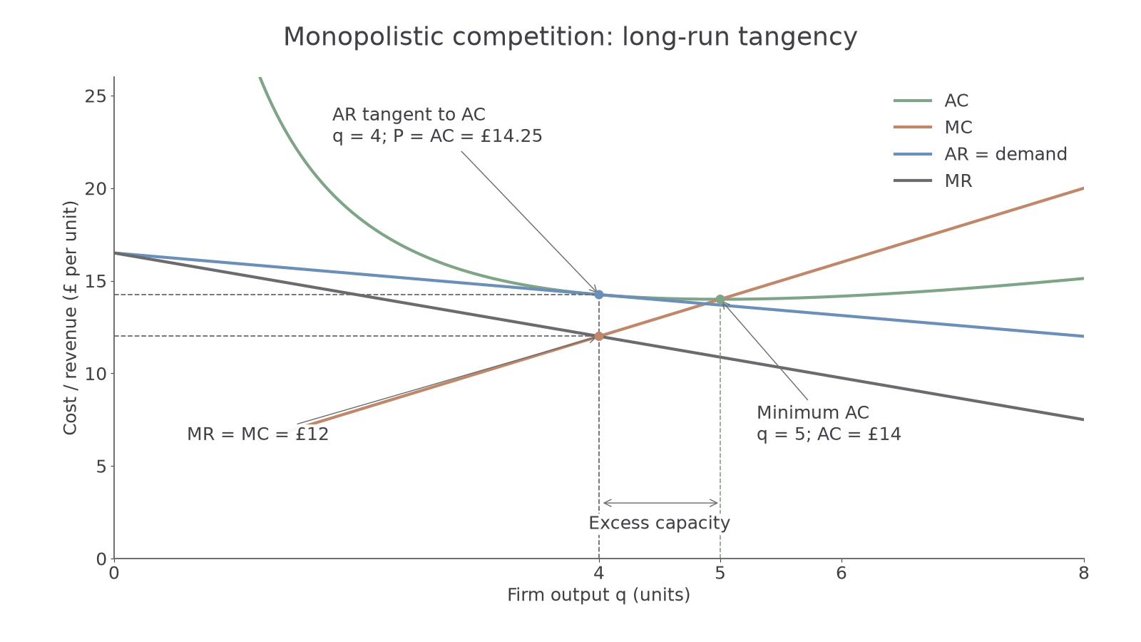
Economic profit encourages other firms to enter when barriers are low. New offers take some customers from the original firm: its demand shifts left, and closer alternatives may also make demand more elastic. Industry demand need not fall; it is demand for each existing firm's offer that is affected.