3.1.3.4 - Price elasticity of supply
Learn to calculate and interpret how strongly quantity supplied responds to price, and explain how time, spare capacity and production conditions change that response.
Calculating supply responsiveness
Price elasticity of supply (PES) measures the proportional responsiveness of quantity supplied to a change in the product's own price, other things equal. It is a ratio of percentage changes, not the extra number of units produced per pound.
For before-and-after calculations in this lesson, use the original value as each denominator:
Illustrative example: the price of garden pots rises from £10 to £12 and quantity supplied rises from 500 to 650 per month, with costs and capacity unchanged.
Quantity responds by 1.5 times the percentage price change over this interval. PES has no currency or quantity unit because the percentage units cancel. For the usual upward-sloping supply curve it is positive. If price and quantity both fall along the same curve, both percentage changes are negative, leaving a positive ratio. Do not automatically add the negative sign associated with ordinary price elasticity of demand.
Dividing 150 pots by £2 gives 75 pots per pound, which measures an absolute response, not elasticity. Dividing by the final rather than the original values also answers a different percentage-change calculation. If a question specifies another convention, such as the midpoint method, follow it; do not silently mix conventions.
A percentage change compares an amount with its starting value. A rise in a percentage measure from 20% to 25% is 5 percentage points, or 25% relative to its original 20%. PES uses percentage changes in price and quantity, not a percentage-point subtraction between unrelated percentages.
Interpreting elasticity values
The magnitude of PES compares the percentage quantity response with the percentage price change.
| PES | Meaning |
|---|---|
| 0 | Perfectly inelastic: quantity cannot respond over the relevant period; a vertical supply curve |
| Between 0 and 1 | Inelastic: quantity changes by a smaller percentage than price |
| 1 | Unit elastic: equal percentage changes |
| Greater than 1 | Elastic: quantity changes by a larger percentage than price |
| Approaches infinity | Perfectly elastic: the idealised horizontal curve offers any relevant quantity at one price |
For example, PES 0.25 means a 12% price rise is associated with a 3% quantity increase over the specified range if the elasticity remains applicable. PES 2 means a 12% rise is associated with a 24% quantity increase. A value of 2 does not mean two extra units, or that output doubled.
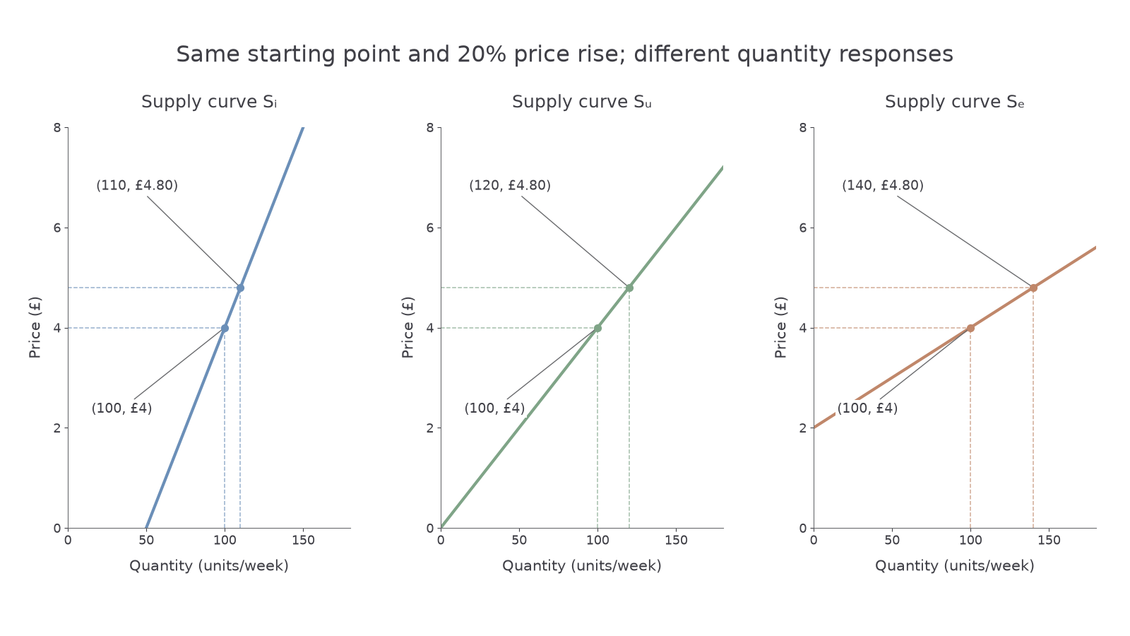
All three illustrative curves pass through the same starting point, £4 and 100 units per week. At £4.80, inelastic Sᵢ offers 110 units, unit-elastic Sᵤ offers 120 and elastic Sₑ offers 140. The common 20% price rise produces quantity increases of 10%, 20% and 40%, hence PES values of 0.5, 1 and 2 respectively over this interval. Read the horizontal intersections at £4.80 rather than judging the labels alone.
To sketch the representation on paper, label price and quantity axes, draw the shared starting point, then draw each curve through its second price–quantity point. A straight supply line through the origin has unit elasticity; straight lines with other intercepts do not necessarily have constant elasticity along their entire length. The stated 0.5 and 2 apply to the selected interval, not every point on Sᵢ and Sₑ. Visual steepness alone is not a reliable elasticity comparison across diagrams with different scales, units or starting points.
A zero change in price gives a zero denominator in the basic before-and-after formula. Do not report an ordinary finite ratio by dividing by zero; the perfectly elastic curve is a limiting model.
Production flexibility and spare capacity
Supply is more elastic when firms can expand output quickly without a large increase in cost. Spare capacity means existing productive resources are not fully used. An empty shift or idle machine lets a firm respond to a higher price with more output; a factory already running continuously may need costly investment before it can expand substantially.
Other constraints affect the percentage response:
- Stocks of finished goods can be released quickly, increasing current supply, but stocks can run out. Storage is harder for perishable goods.
- Readily available inputs and mobile workers make expansion easier. Specialist training, scarce raw materials or unavailable machinery constrain it.
- A short production process allows a quick response. Trees cannot mature or crops be harvested immediately after a price rise.
- Resources that can switch between uses increase flexibility, although expanding one product may reduce supply of another.
Consider two illustrative firms facing a 10% price rise with other conditions fixed. A furniture workshop increases supply from 1,000 to 1,200 units by using an idle machine: a 20% rise, so PES is 2. A workshop at full capacity increases from 1,000 to 1,050 using limited overtime: a 5% rise, so PES is 0.5. These data establish a more elastic response in the first workshop. The stated capacity difference explains a plausible mechanism; in an uncontrolled real comparison, other differences could also matter.
A profitable opportunity and the ability to exploit it are different. High prices do not instantly create trained workers, harvests or additional venue space. Conversely, a larger absolute output increase does not prove higher PES unless the starting quantities and price changes are considered.
Time horizons and market outcomes
The period available to adjust is often decisive for PES. In the immediate period, output may be fixed: a concert cannot add seats on the night. In the short run, firms can change some inputs, such as overtime, while others remain fixed. In the long run, all production inputs can be varied; firms can build capacity and new firms can enter. These are economic adjustment periods, not universal numbers of months.
Illustrative housing application: a rise in the price of new homes can reward building, but land permissions, skilled labour and construction take time. The near-term quantity response may be small. Over several years, more sites and capacity can allow a larger response. Long-run supply is often more elastic, but that is conditional: permanently scarce land, regulation or finite resources can keep it constrained.
When demand increases, a relatively inelastic supply response tends to concentrate the adjustment in price, while an elastic response allows a larger quantity increase. This comparison holds for the same demand change from comparable starting conditions; the equilibrium lesson explains the adjustment mechanism. It does not mean PES causes demand to shift.
Use an estimated elasticity only for the market, period and price range it describes. A factory may initially respond elastically while idle capacity remains, then become less responsive near its capacity limit. A historic PES estimate can therefore be a poor forecast after stocks are exhausted or production conditions change.
When analysing a demand-led price rise, do not call the resulting higher quantity a rightward supply shift: PES describes movement along the existing supply relationship. Investment or new technology may later change that relationship and shift supply. Separate the response to price from the change in production conditions.