3.1.4.3 - Diminishing returns and returns to scale
Learn how output changes when a firm adds one input to fixed capacity, and when it expands all inputs together. Use total, average and marginal product to distinguish diminishing returns from returns to scale and connect them to costs.
Which inputs can change?
The short run is a period in which at least one factor of production is fixed. The long run is a period in which all factors can be varied. These are definitions about flexibility, not fixed calendar lengths.
A café might add staff next week while its kitchen size and equipment remain fixed. This is a short-run adjustment. Once it can choose a different kitchen, equipment and staffing level, it can make a long-run adjustment. For a software service, rented computing capacity may change quickly; building a new port can take years. The relevant period depends on the production process.
A fixed input need not be used fully. An oven can have spare capacity even though the firm cannot yet obtain a different oven. Nor does “long run” mean that every firm actually expands every factor: it means that those choices are available.
To study an input–output relationship, hold other relevant conditions constant. If staff numbers, machinery, product quality and technology all change at once, a change in output alone cannot identify the effect of one extra worker.
Three measures of output
Total product (TP) is the total output produced in a period. Average product (AP) is output per unit of a variable input. Marginal product (MP) is the extra output from an extra unit of that input, keeping the other inputs fixed.
Here is labour input. If workers are added one at a time, the extra output from the fourth worker is . If labour rises by two workers together, divide the change in output by two: that gives marginal product per added worker over the interval, not the separate product of each worker.
This original illustrative table describes one shift with the same equipment and technology throughout.
| Workers | Total product (units per shift) | Average product (units per worker per shift) | Marginal product of added worker (units per shift) |
|---|---|---|---|
| 0 | 0 | Not defined | Not defined |
| 1 | 8 | 8 | 8 |
| 2 | 20 | 10 | 12 |
| 3 | 36 | 12 | 16 |
| 4 | 48 | 12 | 12 |
| 5 | 55 | 11 | 7 |
| 6 | 60 | 10 | 5 |
| 7 | 56 | 8 | −4 |
The fifth worker's marginal product is units; average product with five workers is units per worker. They answer different questions. AP is undefined at zero labour because division by zero is undefined.
The extra worker affects the average in the same way an extra score affects a mean. If MP is above the previous AP, AP rises. If it is below, AP falls. In this discrete example the fourth worker adds 12 units, equal to the previous AP of 12, so AP stays at 12. A smooth production model has MP crossing AP at AP's maximum; discrete data can instead have a tied maximum across observations.
Why marginal returns diminish
The law of diminishing returns states that, as more of a variable input is added to fixed inputs, its marginal product eventually falls, other conditions such as technology held constant. The law concerns marginal output, not an immediate fall in total output.
Initially, extra workers may make better use of idle machinery and allow tasks to be divided. In the table, MP rises from 8 to 12 to 16. Later, workers have to share the same machines and space. Waiting, congestion and coordination reduce the extra output gained from another worker. Diminishing marginal returns begin with the fourth worker: MP falls from 16 to 12.
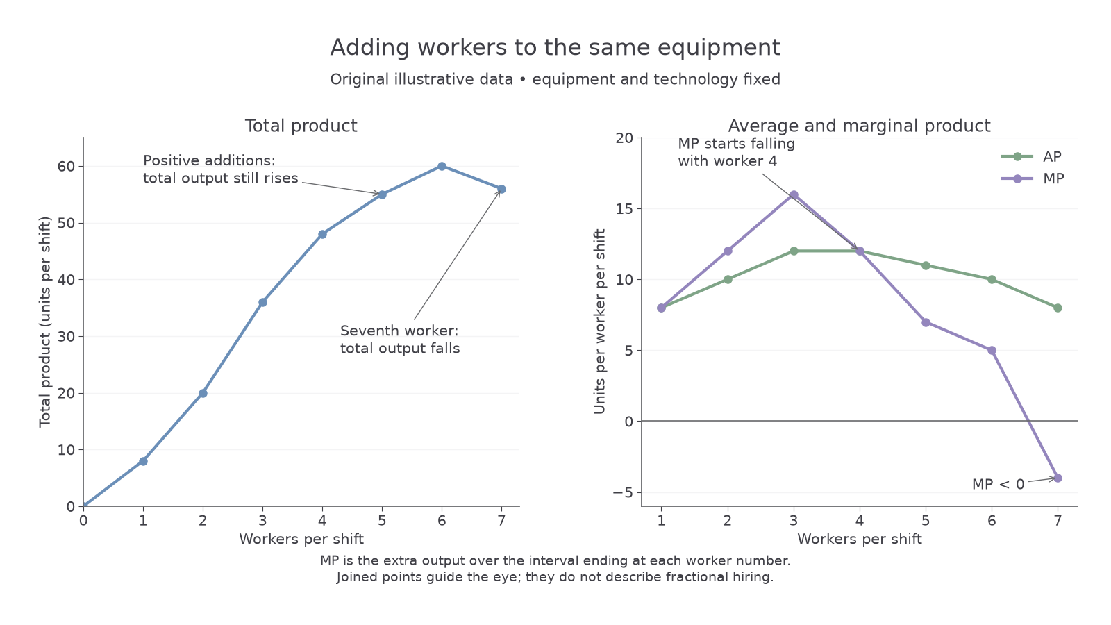
From four to six workers, MP remains positive, so TP still rises from 48 to 60. TP rises more slowly because each extra worker adds less output. At the seventh worker MP is negative, so TP falls to 56. Diminishing returns can therefore occur well before negative returns. AP can also keep rising for a time after MP starts falling, provided MP remains above the previous average.
The diagram uses the table's discrete observations; lines joining points guide the eye. MP is the addition over the hiring interval ending at each worker number. In a smooth model, the slope of TP gives MP, TP is steepest where MP is highest, and TP reaches a maximum where MP is zero.
More or better equipment could change the production relationship. It would be misleading to use the law to claim that labour always becomes less productive regardless of capital or technology.
Expanding all inputs together
Returns to scale describes how output changes when all factor inputs increase in the same proportion, with technology unchanged. It is a long-run comparison because all inputs can vary.
Suppose an original illustrative factory uses five workers and two machines to make 100 units per day. Double every factor, including premises and relevant materials, rather than only the workers. The input scale increases by .
| Output after doubling all inputs | Output change | Returns to scale |
|---|---|---|
| 250 units per day | Increasing | |
| 200 units per day | Constant | |
| 160 units per day | Decreasing |
Increasing returns to scale means output increases more than proportionately; constant returns to scale means the same proportion; decreasing returns to scale means less than proportionately. Decreasing returns still allow total output to increase: 160 is greater than 100, but it is less than the 200 that a proportional increase would produce.
Larger scale can allow deeper specialisation or a more effective arrangement of production. Conversely, coordination problems can make an expanded operation less productive. Returns to scale measures the resulting physical input–output relationship. It does not by itself tell us what happens to wages, machine rental prices or other factor prices.
A rise in labour with machinery unchanged is not a returns-to-scale experiment. It is a change in one input against fixed capacity. A firm can experience diminishing marginal returns to labour in its existing factory yet achieve increasing returns to scale when it expands the whole operation.
What the production relationship means for costs
The physical productivity of an input affects the cost of obtaining an extra unit of output. If an additional worker costs £60 per shift, the third worker in the table adds 16 units at per additional unit. The fourth adds 12 units at ; the sixth adds five at .
With a constant wage, diminishing positive MP means more labour expenditure is needed per additional unit of output. Marginal cost therefore rises in this simple short-run case. This conclusion needs the wage and other relevant costs to be unchanged; rising wages can raise marginal cost even without falling MP. A negative MP is not a cheap way to produce extra output: that worker reduces it.
Returns to scale has a related long-run cost implication. If all factor prices are constant, doubling all inputs doubles the cost of those inputs. If output rises from 100 to 250, cost per unit becomes of its old level, a fall. If output doubles, average cost is unchanged. If output rises only to 160, average cost becomes of its old level, a rise.
Thus increasing returns to scale can support falling long-run average cost at constant factor prices. But a bulk-purchase discount can lower costs without changing the physical returns to scale. Keep the input–output claim separate from the input-price claim.
Quick recap
Diminishing returns adds a variable factor to fixed inputs and tracks marginal product. Returns to scale changes all inputs proportionately and compares the proportional output response. Both describe production, and both affect costs under stated factor-price assumptions.