3.2.2.4 - Aggregate demand and the multiplier
Explain how an initial spending change passes between firms and households, calculate the multiplier from the marginal propensity to consume, and distinguish a simple fixed-price model from an open economy with leakages and capacity constraints.
From spending to income
Changes in AD influence economic activity because firms respond to sales. When there are idle workers and machines, an increase in planned spending can reduce unwanted inventories and prompt higher production. Firms pay additional wages and other incomes, so real national income and employment can rise. If capacity is already tight, extra expenditure may instead raise the price level more than real output.
An autonomous spending change is an initial change not caused by the current change in income, such as a new investment project or a discretionary public purchase. The multiplier process is the subsequent sequence in which that expenditure becomes income, some of which is spent again, generating further income. An identity such as income = expenditure records each transaction; decisions to spend additional income explain the propagation.
Imagine an illustrative £10 million order for domestic construction. Builders receive income; they pay workers and suppliers; recipients spend some of the extra income on other domestic output. Those sellers receive additional income and may spend again. The rounds are not separate duplications of the original building's value: they are further production and purchases induced by new incomes. Counting the original order once and the later distinct output avoids double-counting intermediate inputs.
A spending reduction works in reverse. Cancelled orders reduce incomes, recipients cut some spending, and other firms lose sales. The process can magnify either an increase or a decrease in demand.
The marginal propensity to consume
The marginal propensity to consume (MPC) is the proportion of additional income used for additional consumption:
For a household decision, use additional disposable income in the denominator. If disposable income rises by £200 and consumption rises by £150, MPC is , not £150 and not 75 percentage points. It describes the response to an income change, unlike the average proportion of total income consumed. The remaining additional £50 is saved in this simple household example.
For the simple national multiplier below, income is also disposable income because taxation is omitted. Consumption is entirely on domestic output and there are no imports. If MPC is 0.6, a £10 million initial injection produces induced spending rounds of £6 million, £3.6 million, £2.16 million and so on. Each round is smaller because only 60% of the new income is spent again; the other 40% is saved. The initial injection is included in the total.
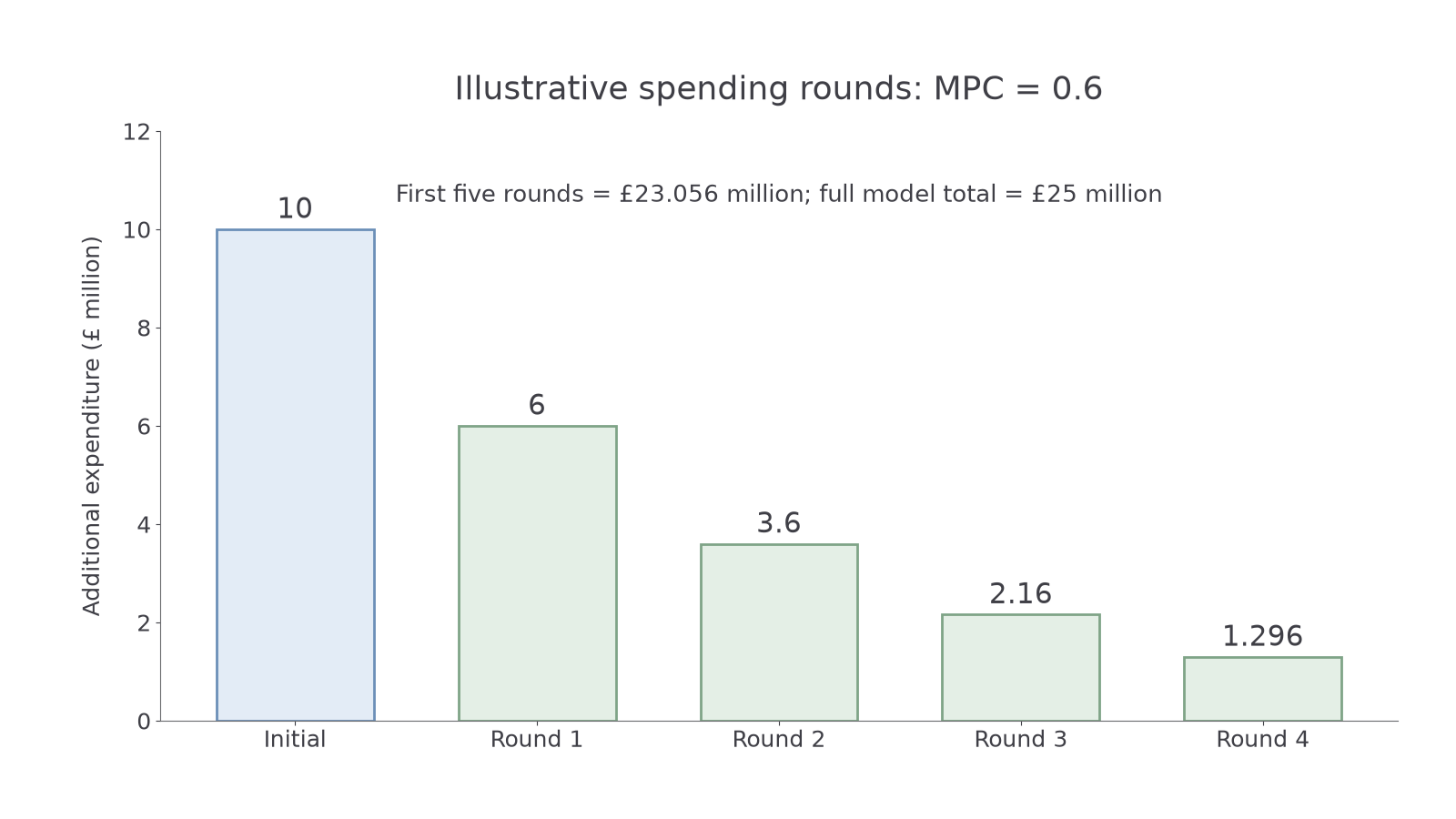
The bars show only the first five rounds, not the full final increase. Their sum is £23.056 million; later positive rounds take the model's total towards £25 million. A higher MPC leaves more spending circulating in every successive round, so the cumulative increase is larger.
Continue this lesson.
You’re previewing NovaLearn without an account. Create a free account to read the rest.
Create free account