3.1.4.4 - Cost curves and factor choices
Learn why total, average and marginal cost curves have their characteristic shapes and how to draw and interpret them consistently. Then explain how factor prices and productivity affect costs and the choice of production inputs.
Total costs and their slopes
A cost curve shows how a cost measure changes with output, holding relevant conditions such as factor prices, technology and the fixed plant constant. A change in output is a movement along that schedule; a change in those conditions can change the schedule itself.
In the standard short-run model, TFC is a horizontal line. TVC starts at zero when no variable inputs are used. TC starts at TFC and remains vertically above TVC by that fixed amount, because .
The slope of TC measures marginal cost in a smooth model. The slope of TVC is the same, because adding a constant fixed cost does not change a curve's slope. With positive MC, both totals rise even when MC is falling. Falling MC means they become less steep, not that their total heights fall.
Initially, better use of fixed equipment and division of labour may raise the marginal product of workers. At a constant wage, less expenditure is required per extra unit, so MC falls and TVC becomes less steep. Eventually, diminishing marginal returns against fixed capacity raise MC, so TVC and TC become steeper. This explains the familiar reverse-S shape of these total curves. It is a model under stated assumptions, not a rule that every measured business cost curve must look identical.
The next section's two-panel diagram uses one consistent original illustrative cost relationship. TFC is £40 per day throughout; TC and TVC never fall. The increasing steepness at higher output matches the rising MC in the other panel.
Average curves and their marginal intersections
The marginal cost of extra output pulls the average towards itself. If MC is below AVC, extra units cost less than the existing average variable cost, so AVC falls. If MC is above AVC, AVC rises. In a smooth model, MC crosses AVC at AVC's minimum. The same logic applies to ATC: MC crosses it at its minimum.
AFC continually falls as fixed cost is spread across more output. Since , ATC lies above AVC, with a gap equal to AFC. The gap narrows as output rises. ATC can keep falling after AVC starts rising because its falling fixed-cost component initially outweighs the variable-cost increase. Its minimum is therefore to the right of AVC's minimum in this model with positive fixed cost.
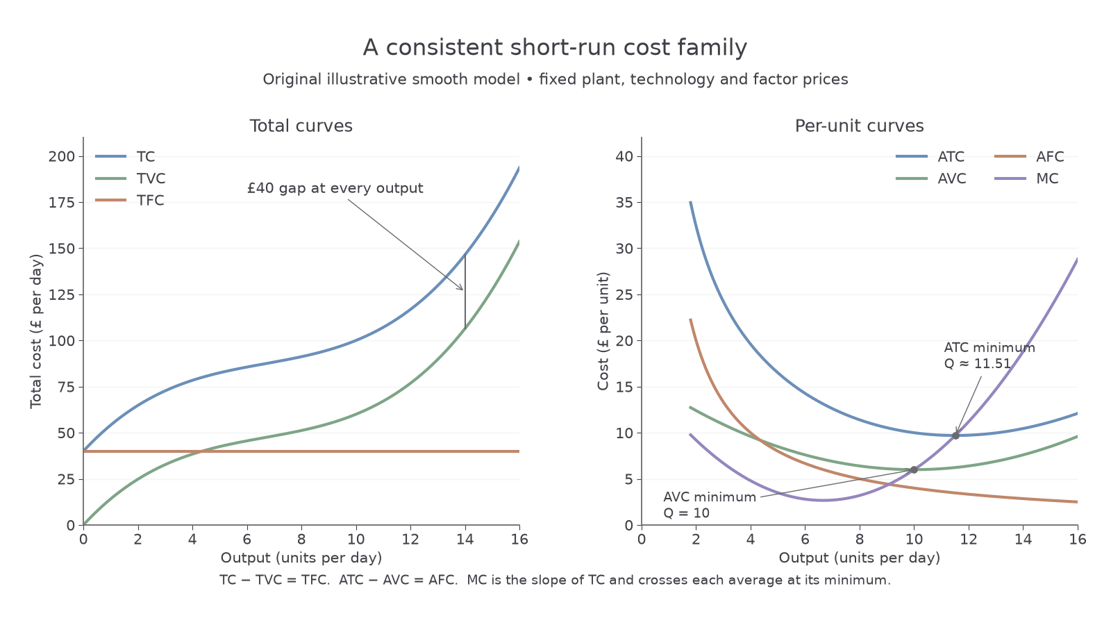
These are original illustrative observations from the smooth relationship in the diagram. MC is supplied at the stated output; it is not an average over the intervals between rows.
| Output (units per day) | TC (£ per day) | AVC (£ per unit) | ATC (£ per unit) | MC (£ per unit) |
|---|---|---|---|---|
| 5 | 82.50 | 8.50 | 16.50 | 3.50 |
| 8 | 91.20 | 6.40 | 11.40 | 3.20 |
| 10 | 100.00 | 6.00 | 10.00 | 6.00 |
| 12 | 116.80 | 6.40 | 9.73 | 11.20 |
| 14 | 146.40 | 7.60 | 10.46 | 18.80 |
AVC reaches its minimum at 10 units. ATC reaches its minimum at about 11.51 units, between the sampled rows; a table's lowest observed value need not be the curve's exact minimum. Between 8 and 10, MC rises from £3.20 to £6 but remains below ATC, so ATC still falls. “MC is rising” is insufficient to conclude “AC is rising”.
To construct these representations in a notebook, use separate vertical axes for totals (£ per day) and averages/marginals (£ per unit), with output per day on both horizontal axes. Plot TFC horizontally at £40, start TVC at zero and keep TC £40 above it. On the per-unit panel, plot a falling AFC and U-shaped AVC and ATC. Draw MC crossing each average at that average's minimum, with the ATC intersection farther right. Use the supplied values and scales rather than drawing unrelated U-shapes. Average curves are undefined at zero output. Label each curve directly or use a clear key.
A notebook drawing develops construction skill. A written interpretation should name the relevant curve, output range and mechanism, rather than merely describe a line as going up or down.
Factor prices and productivity
An input's price and its productivity jointly determine the cost of the output it helps produce. A higher wage does not by itself establish higher labour cost per unit.
Suppose an original illustrative labour-only task pays £18 per hour and produces three identical units per labour hour. Its direct labour cost is per unit. After training, the wage is £24 but output is six per hour; labour cost is per unit. The wage rises by one-third while productivity doubles, so the direct unit cost falls. Include training and other input costs before drawing a conclusion about total production cost.
With unchanged productivity, a higher price of variable inputs raises TVC and TC at each positive output. It also raises AVC and generally MC. A better production method can instead reduce variable inputs needed for a given output and shift these schedules down. Increasing output on the old plant simply moves along the old curves.
A rise in a fixed rent has a different effect. If TFC rises from £40 to £60 with the variable-cost relationship unchanged, TC shifts upward by £20 at every output. AFC and ATC rise by , so the per-unit increase is larger at low output. TVC, AVC and MC are unchanged. At 10 units, ATC rises from £10 to £12, but MC remains £6. Do not shift every cost curve simply because one cost increased.
Productivity gains need not occur uniformly at every output, and factor prices need not stay constant as a firm expands. Identify the changed condition before interpreting a shift.
Choosing a factor combination
A firm choosing inputs compares the cost of producing a specified output and quality using feasible combinations. Cheap labour per hour may require many hours; expensive machinery may produce quickly. Compare the complete resource cost, not just the sticker prices of one worker and one machine.
The following original illustrative methods each produce 100 identical units. Labour costs £15 per hour and machine services £30 per machine hour; all other costs are equal.
| Method | Labour hours | Machine hours | Labour cost | Machine cost | Total relevant cost |
|---|---|---|---|---|---|
| A: more labour | 20 | 2 | £300 | £60 | £360 |
| B: more machinery | 10 | 6 | £150 | £180 | £330 |
B costs £30 less for the same output, despite its greater spending on machine services. If wages rise to £20 with the input requirements unchanged, A costs and B costs . The wage rise strengthens B's cost advantage because it uses fewer labour hours.
Alternatively, keep wages at £15 but raise the machine-service price to £50. A then costs £400 and B £450, making A cheaper. Relative factor prices influence the incentive to substitute between feasible methods.
Substitution depends on technical possibilities and the time available. Machinery may replace one repetitive task while requiring skilled workers to install, operate or maintain it: labour and capital can also be complementary. A new machine may raise the productivity of the remaining workers, and lower costs may allow output to expand. It does not follow that a higher wage always causes immediate automation or that automation always reduces total employment.
Training, installation costs, reliability and uncertain demand matter to the choice. A machine-intensive method can have low operating cost but a large initial commitment that is hard to justify for a short season. In the short run an existing fixed plant can restrict substitution; the long run allows a wider choice. Use the stated assumptions to reach a conditional cost comparison rather than treating one factor combination as universally best.
Quick recap
MC governs the slope of total cost and the direction of average costs. Distinguish movements caused by output from shifts caused by prices or productivity, and distinguish fixed-cost shifts from variable-cost shifts. Input choice compares complete feasible methods under their actual conditions.