RP06 - EMF and Internal Resistance
Every battery you buy is labelled with a voltage, yet connect it to a circuit and a voltmeter across its terminals reads something lower. The difference is not a manufacturing error; it is a fundamental consequence of the battery doing work to push charge through its own materials. Required Practical 6 exploits this effect: by systematically varying the current drawn from a cell and measuring the terminal pd each time, you can extract both the true emf and the internal resistance from a single straight-line graph. The intercept, gradient, controls, and uncertainties determine whether those two values are trustworthy.
1. The Physics Behind the Practical
What you are investigating
You are measuring how the potential difference across the terminals of a cell changes as the current through it increases. From these measurements, you will determine two quantities: the electromotive force (emf) and the internal resistance of the cell.
Electromotive Force (emf)
The emf () of a source is the energy transferred per unit charge by the source when charge passes through it. It is the total voltage the cell provides, measured in volts (V). It equals the terminal pd only when no current flows.
Every real cell is made of chemicals and metal contacts that oppose the flow of charge. This opposition is the internal resistance.
Internal Resistance
The internal resistance () of a source is the resistance within the source itself. It causes a potential difference to be dropped inside the cell whenever current flows, measured in ohms ().
Deriving the key equation
Consider a cell of emf and internal resistance connected to an external resistance . The cell, its internal resistance, and the external resistor are all in series, so the total resistance in the circuit is . The current is therefore:
Current in a Circuit with Internal Resistance
Multiplying both sides by gives the emf equation:
The term is the potential difference across the external resistor, which is what a voltmeter connected across the cell terminals actually reads. We call this the terminal pd, . The term is the potential difference dropped inside the cell, called the lost pd. Substituting :
Terminal pd Equation (the equation you test)
This is the single most important equation for this practical. Read it physically: the terminal pd equals the emf minus whatever voltage is wasted pushing current through the cell's own resistance.
Linearisation for graphical analysis
Compare with the general straight-line equation :
| Straight-line form | This practical |
|---|---|
| (terminal pd) | |
| (current) | |
| (gradient) | (negative internal resistance) |
| (-intercept) | (emf) |
So when you plot terminal pd () on the -axis against current () on the -axis, you get a straight line with:
- -intercept (the emf)
- gradient (the negative of the internal resistance)
The gradient is negative because increasing the current increases the lost pd, which decreases the terminal pd. The -intercept gives the emf because it corresponds to , at which point no energy is lost internally and .
is a straight-line equation. Plotting against gives a line whose -intercept is the emf and whose gradient is . The internal resistance is the magnitude of the gradient.
2. Equipment, Setup, and Method
Equipment list
| Item | Purpose |
|---|---|
| Cell or battery (e.g. 1.5 V D-cell) | The source whose emf and are to be determined |
| Cell holder | Secure electrical contact with the cell |
| Variable resistor (rheostat, e.g. 0--20 ) | Changes the total external resistance to vary the current |
| Digital voltmeter (0--10 V range) | Measures the terminal pd across the cell |
| Digital ammeter (0--1 A range) | Measures the current through the circuit |
| Switch | Allows the circuit to be opened between readings to protect the cell |
| Connecting leads | Complete the circuit |
| Optional: fixed protective resistor (e.g. 1 ) | Limits the maximum current to a safe value when the rheostat is at minimum resistance |
Circuit diagram
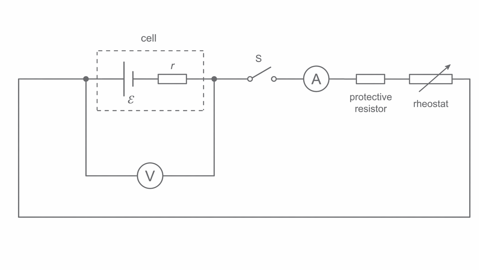
Study the circuit diagram below and notice the two measurement positions that matter most: the voltmeter is connected directly across the cell terminals to read the terminal pd, while the ammeter, switch, and rheostat are all in series to control and measure the current.
[DIAGRAM: asset_name: RP 06 - Investigation of the EMF and Internal Resistance of Electric Cells - Diagram 1; asset_slug: RP 06 - Investigation of the EMF and Internal Resistance of Electric Cells - Diagram 1; recommended_method: retained_png; description: Circuit diagram. A cell (with its internal resistance drawn as a small resistor in series inside a dashed box) is connected in series with a switch (S), a digital ammeter (A), and a variable resistor (rheostat). A digital voltmeter (V) is connected in parallel directly across the terminals of the cell. The voltmeter has a very high resistance, so it draws negligible current. If a protective resistor is used, it sits in series between the ammeter and the rheostat.]
Step-by-step method
-
Connect the circuit as shown in the diagram. Set the variable resistor to its maximum resistance. Ensure the voltmeter is connected directly across the cell terminals (not across the rheostat), so it reads the terminal pd.
-
Open-switch reading. With the switch open, record the voltmeter reading. No current flows, so this reading is approximately equal to the emf. This gives you a check value, though the true emf will be determined more accurately from the graph.
-
Close the switch and immediately read both (voltmeter) and (ammeter). Record the pair of values. Open the switch straight away after taking the readings.
-
Decrease the resistance of the variable resistor by a small, roughly equal step. Close the switch, record and , then open the switch again.
-
Repeat step 4 to collect at least 8--10 pairs of readings, spread across the widest possible range of current. The lowest current corresponds to the rheostat at maximum resistance; the highest current corresponds to minimum resistance.
-
At each rheostat setting, take the reading at least twice and check for consistency. If the two readings differ by more than the resolution of the meter, take a third and use the mean.
-
Record your data in a table with columns for / A and / V, including any repeated readings and calculated means.
Why each step matters
-
Maximum resistance first: Starting at the highest resistance gives the lowest current, which is gentlest on the cell. You then increase the current gradually, which makes it easy to spot if the cell is deteriorating.
-
Open the switch between readings: Continuous current heats the cell internally. This changes the internal resistance (and potentially the emf) during the experiment, introducing a systematic error that makes later readings unreliable.
-
Use a fresh cell: Run-down cells have unstable chemical reactions. Their emf and internal resistance drift during the experiment, meaning the relationship breaks down and your graph will not be a straight line. A fresh cell maintains constant and throughout.
-
Voltmeter directly across the cell terminals: The voltmeter must stay connected across the cell terminals throughout the experiment. That reading is the terminal pd used in . If you move the voltmeter elsewhere in the circuit, you are no longer directly measuring the quantity plotted on the graph.
In a describe-a-method answer, the key chain is simple: measure and , vary the current with the variable resistor, open the switch between readings, plot against , then use the -intercept for emf and the magnitude of the gradient for internal resistance.
3. Variables, Controls, and Experimental Design
| Variable type | Description |
|---|---|
| Independent variable | Current through the cell, varied by adjusting the variable resistor. Range: typically 0.05 A to 0.80 A (depends on the cell used). |
| Dependent variable | Terminal pd across the cell, measured with a digital voltmeter (resolution typically 0.01 V). |
| Control: same cell | Use the same cell throughout. Swapping cells changes both and . |
| Control: temperature of cell | Open the switch between readings to prevent the cell heating up, which would change . |
| Control: connections | Keep all connections tight and unchanged. Loose connections add contact resistance, which would appear as an artificially high . |
| Control: voltmeter position | Keep the voltmeter connected directly across the cell terminals throughout. Moving it changes what is being measured. |
| Control: cell freshness | Use a fresh, unused cell. A partially discharged cell has drifting and . |
Repeats
Take at least two readings of and at each rheostat setting. If they agree within the resolution of the meters, one set is sufficient. If they differ, take a third reading and use the mean. Repeats reduce the effect of random errors in the meter readings.
Ensuring a suitable range
Use a rheostat with a wide resistance range (e.g. 0--20 or 0--50 ) so the current spans from near-zero up to a value where the terminal pd has dropped noticeably (by at least 0.3--0.5 V from the open-switch reading). A wider range of values produces a longer line on the graph, which gives a more accurate gradient and -intercept.
4. Expected Results, Graphs, and Interpretation
Sample results table
The AQA handbook provides two sample readings for a 1.5 V D-cell. Expanding to a realistic full data set gives:
| / A | / V |
|---|---|
| 0.00 (switch open) | 1.62 |
| 0.07 | 1.58 |
| 0.15 | 1.54 |
| 0.22 | 1.50 |
| 0.30 | 1.46 |
| 0.40 | 1.40 |
| 0.50 | 1.35 |
| 0.60 | 1.30 |
| 0.70 | 1.24 |
| 0.80 | 1.19 |
Note: the handbook confirms the two boundary readings: V at mA and V at mA, consistent with V and .
The graph
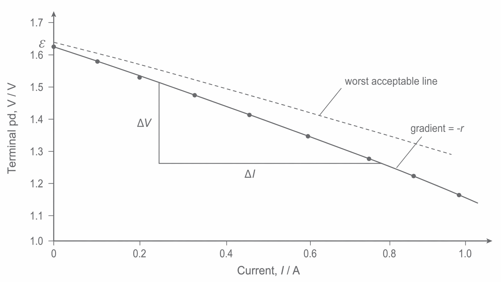
Plot (terminal pd / V) on the -axis against (current / A) on the -axis. The data should form a straight line with a negative gradient, intercepting the -axis above zero.
Look carefully at the graph below: the -intercept gives the emf, the downward gradient gives , and the large gradient triangle plus dashed worst acceptable line show how you extract the internal resistance and its uncertainty clearly from the best-fit trend.
[DIAGRAM: asset_name: RP 06 - Investigation of the EMF and Internal Resistance of Electric Cells - Diagram 2; asset_slug: RP 06 - Investigation of the EMF and Internal Resistance of Electric Cells - Diagram 2; recommended_method: retained_png; description: A V-I graph. The y-axis is labelled "Terminal pd, / V" ranging from about 1.0 to 1.7. The x-axis is labelled "Current, / A" ranging from 0 to about 1.0. Data points fall on a straight line sloping downward from upper-left to lower-right. The line of best fit is drawn through the points. The y-intercept is labelled "" at approximately 1.62 V. A large gradient triangle is drawn spanning at least half the line, with the vertical side labelled "" and the horizontal side labelled "". An annotation reads "gradient ". A dashed "worst acceptable line" is drawn through the outermost data points to indicate uncertainty in the gradient.]
Extracting the physical quantities
-
EMF (): Read the -intercept directly from the graph. This is where the line of best fit meets the -axis (i.e. at ). This value is the emf because when no current flows, .
-
Internal resistance (): Calculate the gradient of the line of best fit using a large gradient triangle (spanning at least half the line length):
The gradient is negative. The internal resistance is the magnitude:
Physical explanation of the trend
As the current increases, more charge flows through the cell per second, so more energy per second is dissipated against the internal resistance. The lost pd () increases, leaving less voltage available at the terminals. The relationship is linear because is constant (for a fresh cell at constant temperature), so decreases uniformly with .
5. Worked Example — Full Calculation
Using the sample data from Part 4, here is a complete walk-through of the analysis.
Step 1: Plot the graph
Plot the nine data points (excluding the open-switch reading, which is at and can be plotted as an additional check). Draw the line of best fit.
Step 2: Determine the emf from the -intercept
The line of best fit intercepts the -axis at:
Step 3: Calculate the gradient
Choose two points on the line of best fit (not raw data points) that are far apart. Using the points and :
Step 4: Determine the internal resistance
Step 5: Compare with the accepted value
The AQA handbook states the expected values are V and . Our graphical analysis gives:
These are in excellent agreement.
Step 6: Verify with a data check
Pick any data point from the table and verify it is consistent with the determined values. Using the point A:
The table shows V at A, which matches perfectly.
Alternative: algebraic method from two data points
If no graph is available, you can use any two pairs. From the terminal pd equation written for each:
Subtracting the second from the first:
Internal Resistance from Two Data Points
Using the AQA handbook boundary readings: V at A, and V at A:
Then substituting back: V.
Both methods converge on the same answer, confirming the analysis.
6. Uncertainty and Error Analysis
This section is critical for AQA Physics. Examiners expect you to identify specific errors for this practical, quantify uncertainties, and suggest meaningful improvements.
Systematic errors
Systematic errors shift all readings in one direction. In this practical:
-
Cell heating: If the switch is left closed, the cell warms up, increasing its internal resistance. This means the lost pd is larger than expected, so the terminal pd readings are systematically too low at higher currents. The gradient becomes steeper (overestimating ) and the emf reading may also drift.
-
Run-down cell: A partially discharged cell has internal chemical changes that cause to decrease during the experiment. Early readings reflect a higher emf than later readings, producing a curved graph rather than a straight line. The result is that both and are unreliable.
-
Meter loading: Real meters are not ideal. A digital voltmeter has a very large but finite resistance, so it draws a tiny extra current in parallel with the external circuit. The ammeter measures the current in the main load branch, so the true current supplied by the cell is very slightly larger than the ammeter reading. A real ammeter also has a small internal resistance, which slightly reduces the current drawn. In practice, with typical digital meters, both effects are negligible compared with the main experimental uncertainties.
Random errors
Random errors cause scatter around the line of best fit:
- Fluctuations in meter readings: Digital meters may fluctuate in the last digit, particularly if the current is not perfectly steady.
- Contact resistance variations: Slightly loose connections can change from reading to reading, adding random scatter.
- Timing of readings: If the switch is held closed for slightly different durations each time, the cell temperature differs, adding random variation.
Worked uncertainty calculation
Suppose the digital ammeter has a resolution of 0.01 A and the digital voltmeter has a resolution of 0.01 V.
Absolute uncertainty in each measurement:
These reading uncertainties come from the meter resolution. Do not confuse them with meter loading: loading is a separate systematic effect caused by the non-ideal resistances of the meters themselves.
Percentage uncertainty in a single reading:
For a mid-range reading of A:
\text{% uncertainty in } I = \frac{0.01}{0.40} \times 100 = 2.5\%For the corresponding V:
\text{% uncertainty in } V = \frac{0.01}{1.40} \times 100 = 0.71\%Uncertainty in the gradient (internal resistance):
Draw the worst acceptable line on your graph. This is the steepest (or shallowest) line that still passes through the error bars of the data points. Calculate its gradient.
Suppose the best-fit gradient is and the worst acceptable line gradient is :
\text{% uncertainty in } r = \frac{0.06}{0.54} \times 100 = 11\%Uncertainty in the emf (-intercept):
The best-fit intercept is 1.62 V. If the worst acceptable line gives an intercept of 1.65 V:
When describing uncertainty in a gradient, refer to the best-fit line and the worst acceptable line through the error bars. The meter resolution sets the size of the error bars, but the uncertainty in comes from how much the gradient can vary while still fitting the data.
Sources of error and improvements table
| Source of error | Type | Effect | Improvement |
|---|---|---|---|
| Cell heats up during readings if switch left closed | Systematic | increases during experiment, so terminal pd drops more than expected at high currents; gradient becomes steeper, overestimating | Open the switch between every pair of readings; only close it for the few seconds needed to read and |
| Using a run-down or old cell | Systematic | Emf and internal resistance drift during experiment; graph is curved, not straight | Use a fresh, unused cell; check the open-circuit voltage before starting |
| Fluctuations in digital meter readings | Random | Scatter in and values; points deviate from the line of best fit | Take repeat readings at each rheostat setting and use the mean |
| Loose or corroded connections | Random | Contact resistance varies unpredictably, adding scatter to both and | Ensure all connections are tight; use clean, bare wire ends; check connections before starting |
| Narrow range of current values | Random (amplifies effect) | Few data points clustered in a small region; line of best fit is poorly defined, leading to large uncertainty in gradient and intercept | Use a rheostat with a wide resistance range; include a protective resistor to safely extend the current range |
| Heating of the variable resistor at high currents | Systematic | Resistance of the rheostat changes as it heats, so the current at a given setting drifts | Use a rheostat with an adequate power rating; take readings quickly |
7. Exam Context — How AQA Tests This Practical
RP06 connects circuit setup, graphical analysis, uncertainty, and evaluation, so it can be approached from several angles.
Question types you should expect
1. "Describe a method" (6 marks): You are given apparatus and told to determine the emf and internal resistance. Full marks require: circuit diagram or description, what to measure ( and ), how to vary the current (variable resistor), opening the switch between readings, plotting against , and extracting from the -intercept and from the magnitude of the gradient.
2. Data analysis: You are given a table of and values and asked to plot a graph, determine the gradient and intercept, and hence find and . You may be asked to draw error bars and a worst acceptable line.
3. Calculation from two data points: Given two pairs, calculate and algebraically.
4. Evaluate the method: Identify sources of error, explain their effect, and suggest improvements. This is where the table in Part 6 earns its marks.
5. Adapt the method: You may be asked how to modify the experiment for a different cell, or how to investigate how internal resistance depends on temperature.
Command words to expect
- Describe: Give a step-by-step account of the method, measurements, and analysis.
- Explain: Give reasons. For example, "Explain why the terminal pd decreases as current increases" requires you to link to the increasing lost pd.
- Calculate: Show your working, give the answer to an appropriate number of significant figures, and include the unit.
- Evaluate: Identify strengths and weaknesses of the method, with specific reference to errors and improvements.
- Suggest: Propose a change to the method and explain why it would improve accuracy or precision.
Adapting the method
A common variant asks you to use fixed resistors instead of a variable resistor. In this case, you swap in resistors of known value one at a time. The method is otherwise identical: measure and for each resistor, plot against , and extract and from the graph. Another variant asks you to investigate how the internal resistance of a cell changes with temperature by placing the cell in a water bath and repeating the experiment at different temperatures.
Battery management systems in electric vehicles continuously monitor the internal resistance of each cell in the battery pack. A rising internal resistance indicates cell degradation. By applying a known current pulse and measuring the voltage drop, the system calculates in real time using the same principle as this practical: . Cells with excessive internal resistance are flagged for replacement before they overheat or fail.
Common student mistakes
- Confusing gradient with : The gradient is , not . Students who forget the negative sign and write lose the mark. State .
- Using raw data points for the gradient instead of the line of best fit: Always take the gradient from two points on the line, not from the data table.
- Forgetting to open the switch between readings: In a describe-a-method question, this is an expected mark-earning point.
- Extrapolating wildly: If your data only covers to A, acknowledge that the -intercept involves extrapolation, which adds uncertainty. The more data points close to , the more reliable the intercept.
- Omitting units: must be in and in V.
- Mixing up emf and terminal pd: Emf is the -intercept (at ); terminal pd is any specific reading from the voltmeter when current flows.
Links to other specification points
- 3.5.1.3 (Resistivity): Understanding resistance and how it depends on material and geometry.
- 3.5.1.4 (Circuits): Series and parallel combinations, Kirchhoff's laws, and how total circuit resistance determines current.
- 3.5.1.5 (Potential divider): If the external circuit is a potential divider, the terminal pd of the cell feeds the divider, and internal resistance affects the output.
- 3.5.1.6 (EMF and internal resistance): The theory behind this practical, including the power equation .
Now test yourself with the most important type of exam question for this practical: the 6-mark extended response.
The ability to describe this method clearly and completely is perhaps the single most valuable exam skill for this practical. Practise writing it from memory.