RP02 - Interference Effects
RP02 turns the interference ideas from Topic 3.3.2.1 into measurements. You will set up Young's double slit and a diffraction grating, collect data that can be graphed, and use those graphs to determine the wavelength of laser light. The theory still matters, but this lesson is mainly about the practical: what you measure, why the graph works, and how to judge which method gives the more reliable wavelength.
Part 1 — Retrieval and the Physics Behind RP02
Why interference happens
When two or more waves overlap in space, the resultant displacement at any point is the vector sum of the individual displacements. This is the principle of superposition. Where crests meet crests (waves arrive in phase), constructive interference produces a bright fringe. Where crests meet troughs (waves arrive exactly half a wavelength out of phase), destructive interference produces a dark fringe.
Those two conditions are the retrieval step that anchors the whole practical. RP02 is really about turning them into quantities you can measure on a screen: fringe spacing for the double slit, and diffraction angles for the grating.
Coherence
Two sources are coherent if they emit waves of the same frequency with a constant phase difference. Coherence is essential for a stable, observable interference pattern — without it, the positions of constructive and destructive interference shift randomly and no fringes are seen.
Laser light is coherent and highly monochromatic, so it can illuminate a double slit directly without needing a preliminary single slit. A non-laser source (filament lamp, LED) requires a narrow single slit first to act as a point-like source, creating spatial coherence before the light reaches the double slit.
Young's double slit — the equation
Consider two narrow slits separated by distance , with a screen placed a large distance away. Light diffracts through each slit and the two diffracted beams overlap on the screen. At a point P on the screen displaced from the central axis, the waves from the two slits travel slightly different distances. The extra distance travelled by one wave relative to the other is the path difference.
Path Difference
The difference in distance travelled by two waves from their respective sources to the same point. For constructive interference the path difference equals a whole number of wavelengths (, where ). For destructive interference it equals .
For the th bright fringe at position from the central maximum, geometry gives the path difference as . When (which is always true in this experiment), the small-angle approximation applies and . Setting the path difference equal to :
Full derivation. Consider slits and and a point P on the screen at the th bright fringe, distance from centre O. Mark a point Q on such that ; then the path difference is . Triangles and the triangle formed by the midpoint M of the slits, O, and P are similar (valid because ):
The fringe separation is the distance between adjacent bright fringes, so . Cancelling and rearranging:
Young's Double Slit Equation
where = fringe separation (m), = wavelength (m), = slit-to-screen distance (m), = slit separation (m).
This equation tells you three things immediately: fringes get wider if you increase , increase , or decrease . Each of these is a common exam question.
Linearisation for graphical analysis
Rearranging the double slit equation for graphical analysis, treat as the independent variable (the quantity you change) and as the dependent variable (the quantity you measure):
This has the form with , , gradient , and (the line passes through the origin). Therefore:
Wavelength from Gradient — Double Slit
A straight line through the origin confirms that is directly proportional to , validating the model. If the line does not pass through the origin, a systematic error is present — most likely a zero error in (measuring from the wrong reference point).
Diffraction grating — the equation
A diffraction grating consists of thousands of equally spaced slits (typically 300 to 600 lines per mm). Each slit acts as a source of coherent secondary wavelets. Because there are so many slits, constructive interference is extremely sharply defined — the bright maxima are narrow and intense, making angle measurements far more precise than with Young's double slit.
Diffraction Grating Equation
where = grating spacing (m), = angle of the th-order maximum from the central beam, = order number (0, 1, 2, ...), = wavelength (m).
The grating spacing is calculated from the number of lines per metre : . For example, a grating labelled "300 lines per mm" has lines m, so m.
Why are grating fringes so much sharper than double slit fringes? With only two slits, the condition for constructive interference is satisfied over a broad angular range, producing wide, fuzzy bright bands. With thousands of slits, even a tiny deviation from the exact angle causes the waves from distant slits to be out of phase, so destructive interference is almost total everywhere except at the precise angles satisfying . The result is bright, narrow lines separated by broad dark regions.
The maximum observable order is limited by the fact that cannot exceed 1:
where means round down to the nearest integer.
Diffraction gratings are the core component of optical spectrometers used in astronomy. When starlight passes through a grating inside a spectrograph, each chemical element in the star's atmosphere produces emission or absorption lines at characteristic wavelengths. By measuring the precise angles of these lines, astronomers determine the chemical composition, temperature, and radial velocity of stars billions of light-years away.
Part 2 — Equipment, Setup, and Method
A: Young's double slit experiment
Equipment list:
| Item | Purpose |
|---|---|
| Class II helium-neon laser (< 1 mW output) | Provides coherent, monochromatic light source |
| Double slit slide (~0.1 mm slit separation) | Creates two coherent secondary sources |
| Adjustable single slit (optional) | Narrows beam if laser is too wide; ensures both slits are illuminated evenly |
| White screen (matt paper on wall or board) | Displays fringe pattern; matt finish prevents specular reflection of the beam |
| Metre ruler (mm scale) | Measures slit-to-screen distance and total fringe span |
| Vernier callipers or travelling microscope | Measures slit separation if not printed on the slide |
| Retort stand with boss and clamp | Holds double slit slide at laser beam height |
| Set square | Ensures screen is perpendicular to laser beam |
Step-by-step method:
-
Darken the room partially. Complete darkness is not necessary with a laser, but reducing ambient light makes fringes much easier to see and measure. The fringe intensity is low and stray light would wash out the contrast between bright and dark fringes.
-
Mount the laser on the bench so it points horizontally toward the white screen. Place the double slit slide in a clamp approximately 0.5 m from the screen.
-
Align the laser beam so it illuminates both slits evenly. Adjust the laser height and angle so the beam spreads across the full width of the double slit. A clear pattern of bright and dark fringes should appear on the screen. If only one slit is illuminated, you get single-slit diffraction instead of two-slit interference — the fringes will be broad and unevenly spaced rather than regularly spaced and uniform.
-
Use a set square to check the screen is perpendicular to the laser beam. If the screen is angled, the fringe spacing on one side of the pattern will differ from the other side, introducing a systematic error. Place the set square flat on the bench with one edge against the screen and sight along the other edge toward the laser.
-
Set the initial slit-to-screen distance m. Measure from the plane of the double slit slide to the screen surface using the metre ruler. Record this value.
-
Measure the fringe separation . Rather than measuring a single fringe width (which would have a large percentage uncertainty), measure the distance across as many fringes as are clearly visible — say 10 bright fringes. Mark the centre of the first bright fringe and the centre of the eleventh bright fringe with a pencil on the screen paper. The distance between these marks spans 10 fringe widths. Divide the total distance by 10 to obtain .
When you count fringes, count the gaps between them rather than the number of bright lines. Measuring from the 1st to the 11th bright fringe gives 10 fringe widths, not 11, and being explicit about that avoids the most common practical mistake in this method.
-
Increase by 0.10 m increments up to m. At each distance, repeat the fringe width measurement. This gives up to 11 data points spanning a wide range — essential for a reliable graph.
-
Repeat the entire set of measurements at least twice more to obtain three values of at each . Calculate the mean for each distance. Repeats allow you to identify anomalous readings and reduce the effect of random errors.
-
Measure the slit separation . If the value is printed on the slide, record it. If not, use vernier callipers (resolution mm) or a travelling microscope to measure the centre-to-centre distance between the two slits. Take at least three measurements and use the mean.
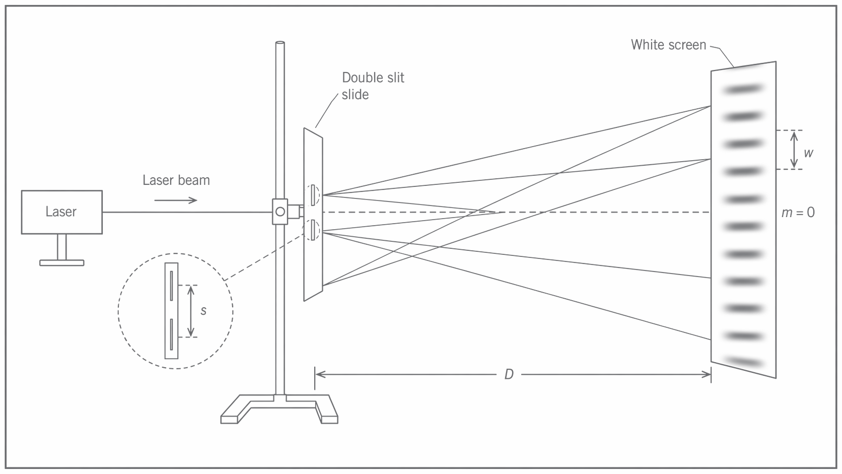
The figure below shows the full double-slit setup; notice where the practical measurements come from by tracking the slit-to-screen distance , the slit separation , and the fringe spacing on the screen.
[DIAGRAM: asset_name: RP 02 - Investigation of Interference Effects - Diagram 1; asset_slug: RP 02 - Investigation of Interference Effects - Diagram 1; recommended_method: retained_png; description: Young's double slit apparatus — laser on the left emitting a horizontal beam, passing through a double slit slide mounted on a retort stand, with diverging overlapping beams hitting a white screen on the right. Label the slit-to-screen distance (horizontal arrow from slit to screen), the slit separation (vertical double-headed arrow at the slit, magnified in an inset), and the fringe separation (vertical double-headed arrow between adjacent bright fringes on the screen). Show alternating bright and dark bands on the screen, with the central maximum labelled .]
B: Diffraction grating experiment
Equipment list:
| Item | Purpose |
|---|---|
| Class II helium-neon laser (< 1 mW output) | Provides coherent, monochromatic light source |
| Plane transmission diffraction grating (e.g. 100 lines mm) | Produces sharp, well-separated diffraction orders |
| White screen (matt paper on wall or board) | Displays diffraction pattern |
| Metre ruler (mm scale) | Measures grating-to-screen distance and order positions |
| Retort stand with boss and clamp | Holds diffraction grating perpendicular to beam |
| Set square | Ensures grating is normal to laser beam |
Step-by-step method:
-
Darken the room partially as before.
-
Mount the diffraction grating in a clamp so the laser beam passes through it at normal incidence (perpendicular to the grating surface). Use a set square to check alignment. If the grating is not perpendicular, the angles of the orders on either side of the central maximum will be unequal, introducing a systematic error.
-
Set m (or similar measured distance). Measure from the grating to the screen with the metre ruler.
-
Observe the diffraction pattern. A bright central spot (zero-order maximum, ) appears with symmetric bright spots on either side — the first order (), second order (), and so on. The number of visible orders depends on and : since cannot exceed 1, the maximum order is the largest integer satisfying .
-
For each order , measure the distance from the central maximum to the th order spot on both sides of the central maximum. Call these and . Average them: . Measuring on both sides and averaging eliminates any error caused by the grating being slightly off-perpendicular.
-
Calculate the angle for each order: .
-
Calculate for each order: .
-
Average the values across all orders to obtain a final result.
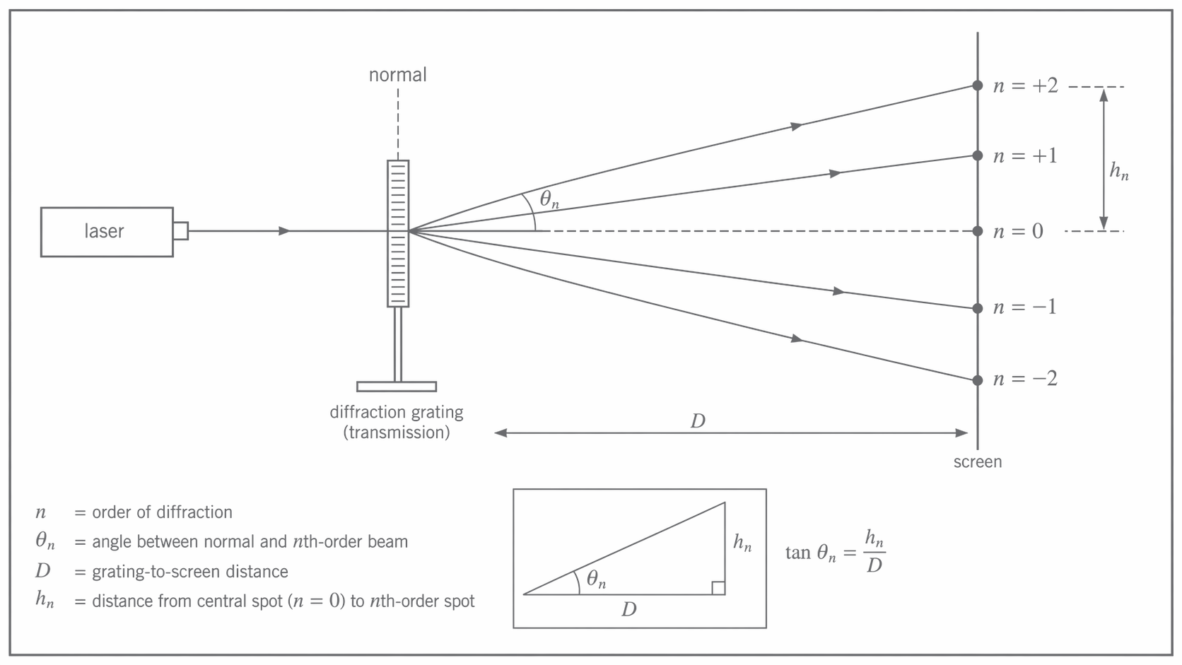
The figure below highlights the measurement geometry for the grating method; notice the fixed distance , the vertical displacement of an order from the centre, and the angle measured from the normal.
[DIAGRAM: asset_name: RP 02 - Investigation of Interference Effects - Diagram 2; asset_slug: RP 02 - Investigation of Interference Effects - Diagram 2; recommended_method: retained_png; description: Diffraction grating apparatus — laser on the left, beam passing through a transmission diffraction grating mounted vertically on a stand, with multiple beams emerging at different angles hitting a screen on the right. Label the grating-to-screen distance (horizontal), the distance from the central spot to the th order spot (vertical), and the angle (measured from the normal to the grating). Show the zero order at the centre, first orders symmetrically placed, second orders further out, with the angle triangle (, , ) clearly marked.]
Safety
Laser safety is critical in this experiment. A Class II laser (< 1 mW) is standard for school use, but it can still cause retinal damage if the beam enters the eye directly or after specular reflection.
- Never look along the beam, even at an angle — specular reflections from glass, polished metal, or even a watch face can redirect the beam into your eye.
- Keep the laser beam horizontal and below eye level of anyone standing in the room.
- Display a laser safety warning sign on the laboratory door.
- Remove shiny objects (jewellery, phones, belt buckles) from the beam path to prevent specular reflections.
- Switch off the laser when not taking measurements to minimise exposure time.
Part 3 — Variables, Controls, and Experimental Design
A: Young's double slit
| Variable type | Description |
|---|---|
| Independent variable | Slit-to-screen distance , varied from 0.50 m to 1.50 m in 0.10 m steps |
| Dependent variable | Fringe separation , measured with a metre ruler (resolution mm) by measuring across multiple fringes and dividing |
| Controlled variable 1 | Slit separation — use the same double slit slide throughout; if changed, the proportionality constant changes and the graph gradient is meaningless |
| Controlled variable 2 | Wavelength — use the same laser throughout; different lasers have different wavelengths |
| Controlled variable 3 | Alignment of screen perpendicular to beam — check with set square at each ; tilting the screen distorts the projected fringe spacing |
| Controlled variable 4 | Room lighting — keep the same level of darkening throughout; brighter ambient light makes fringes harder to see consistently |
| Controlled variable 5 | Ruler position relative to the fringe pattern — always measure from the same reference point (e.g. always from the central maximum outward) |
Repeats: At each value of , measure at least three times (repositioning the ruler each time) and calculate the mean. This reduces the effect of random error in identifying fringe centres.
Range: should span at least a factor of 3 (e.g. 0.50 m to 1.50 m). Too short a range compresses the data points on the graph and makes the gradient unreliable. Too long a range may cause fringes to become too faint to measure at large (the light spreads over a larger area).
B: Diffraction grating
| Variable type | Description |
|---|---|
| Independent variable | Order number ( up to the maximum visible order) |
| Dependent variable | Angle to each order, determined by measuring and then calculating |
| Controlled variable 1 | Grating spacing — use the same grating throughout |
| Controlled variable 2 | Wavelength — same laser as before |
| Controlled variable 3 | Grating-to-screen distance — keep fixed; if changes between measurements, the values are not directly comparable |
| Controlled variable 4 | Normal incidence — grating must remain perpendicular to beam; verify with set square |
For the double slit, one of the key practical choices is to measure across many fringes rather than just one. That increases the total measured distance, so the percentage uncertainty in falls even though the ruler reading uncertainty stays the same.
Part 4 — Expected Results, Graphs, and Interpretation
A: Young's double slit — sample results
The AQA handbook provides the following sample data, collected with a double slit of separation mm m:
| / m | / mm | (calculated) / nm |
|---|---|---|
| 0.50 | 3.11 | 622.0 |
| 0.70 | 4.44 | 634.3 |
| 0.90 | 5.66 | 628.9 |
| 1.00 | 6.27 | 627.0 |
| 1.30 | 8.21 | 631.5 |
| 1.50 | 9.42 | 628.0 |
Notice how the calculated wavelength hovers around 628 nm at each distance — this consistency is evidence that the method is valid and the relationship holds. The scatter (622 to 634 nm) reflects the random uncertainty in measuring .
The graph: plot (in mm) on the -axis against (in m) on the -axis. The relationship predicts a straight line through the origin.
The graph below shows what that straight-line result should look like; notice that the best-fit line runs close to the origin and that the gradient triangle uses two widely separated points on the line rather than raw data points.
[DIAGRAM: asset_name: RP 02 - Investigation of Interference Effects - Diagram 3; asset_slug: RP 02 - Investigation of Interference Effects - Diagram 3; recommended_method: retained_png; description: Graph with / m on the -axis (range 0 to 1.6 m) and / mm on the -axis (range 0 to 10 mm). Six data points plotted forming a clear straight line passing through or very close to the origin. A best-fit line is drawn through the points. A gradient triangle is marked using two well-separated points on the line, with (vertical side) and (horizontal side) clearly labelled.]
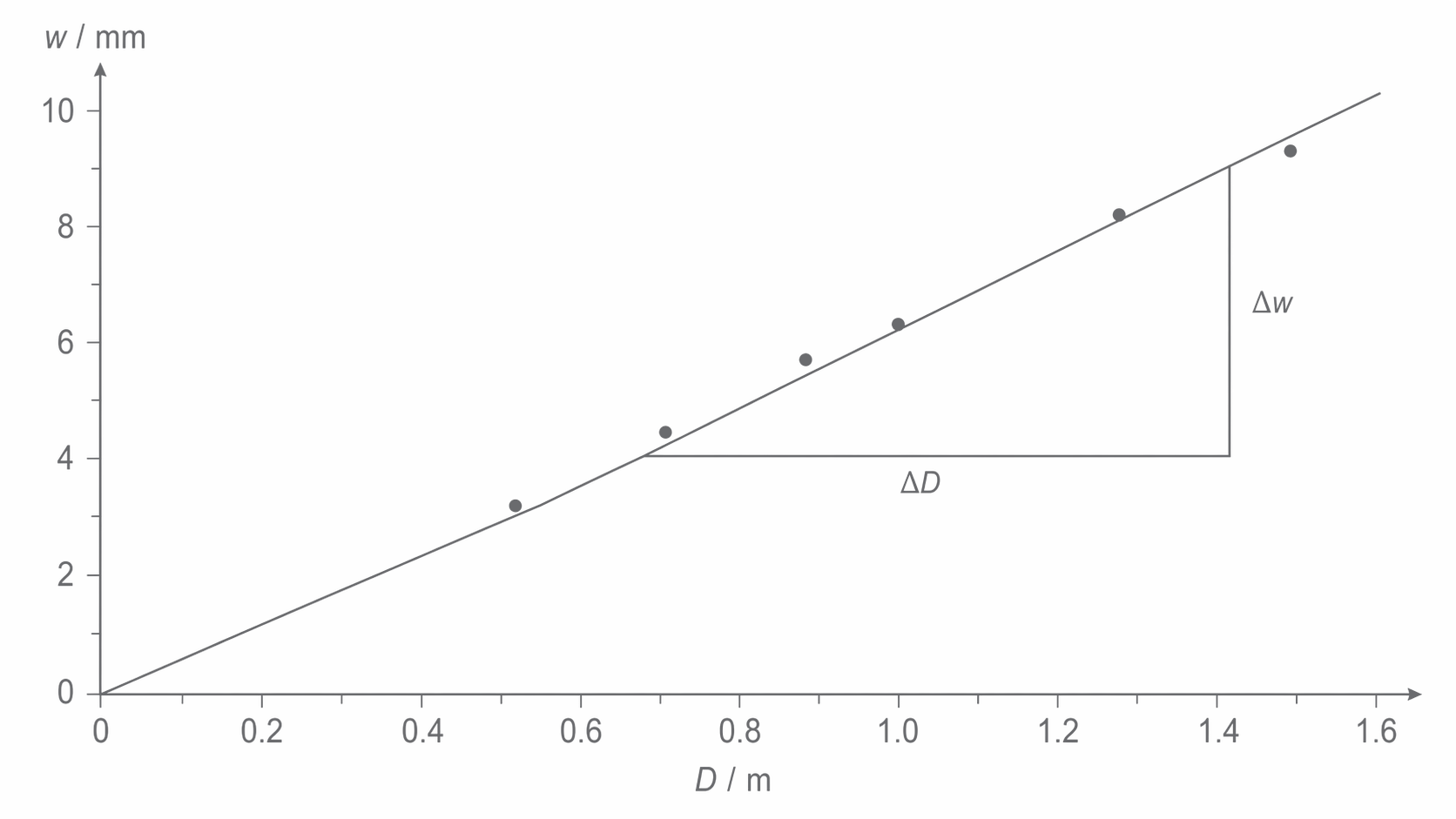
The gradient of the best-fit line gives , so:
B: Diffraction grating — sample results
The AQA handbook provides the following data, collected with m. The grating spacing can be inferred from the results: m (i.e. 100 lines mm).
| Order | / mm | / ° | / nm | ||
|---|---|---|---|---|---|
| 1 | 68.2 | 0.0626 | 3.58 | 0.0624 | 624.5 |
| 2 | 138.4 | 0.1270 | 7.24 | 0.1260 | 629.8 |
| 3 | 208.6 | 0.1914 | 10.84 | 0.1881 | 626.6 |
| 4 | 282.4 | 0.2591 | 14.53 | 0.2510 | 627.0 |
The wavelength values are remarkably consistent across orders (624.5 to 629.8 nm), which is a hallmark of the grating method's precision. Averaging gives nm.
For the grating, you can also produce a linearised graph. Since , rearranging gives:
Plotting on the -axis against on the -axis gives a straight line through the origin with gradient , so:
Wavelength from Gradient — Diffraction Grating
This linearisation is particularly clean: is an exact integer (no uncertainty at all), so every bit of scatter on the graph comes from the uncertainty in . This makes error analysis straightforward and is a favourite exam question.
The physical explanation for the trend is direct: higher orders correspond to larger path differences between adjacent slits ( instead of ), which requires a larger angle for the waves to arrive in phase.
Part 5 — Worked Example: Full Calculation
A: Young's double slit — graphical method
Given data (from the AQA sample results):
| / m | / mm |
|---|---|
| 0.50 | 3.11 |
| 0.70 | 4.44 |
| 0.90 | 5.66 |
| 1.00 | 6.27 |
| 1.30 | 8.21 |
| 1.50 | 9.42 |
Slit separation: mm m.
Step 1: Plot against .
Place on the -axis (range 0 to 1.6 m) and on the -axis (range 0 to 10 mm). The points should lie close to a straight line through the origin.
Step 2: Draw the best-fit line.
Using a transparent ruler, draw the straight line that best represents the trend. It should pass through or very close to the origin (since the equation predicts when ).
Step 3: Calculate the gradient.
Choose two points on the best-fit line that are far apart (use points on the line itself, not necessarily data points). For example, reading from the line:
- At m, mm
- At m, mm
Convert to consistent units: gradient m m (dimensionless ratio when and are both in metres).
Step 4: Calculate the wavelength.
Step 5: Sense-check the value.
A wavelength of m is in the red part of the visible spectrum, which is sensible for the laser used in this practical and consistent with the measured fringe spacing.
B: Diffraction grating — worked calculation for one order
Given data: m, order , distance from central maximum mm, grating spacing m.
Step 1: Calculate the angle.
Step 2: Calculate .
Note that in general. At small angles they are approximately equal, but at larger angles (higher orders) the distinction matters. Always use in the grating equation, not .
Step 3: Calculate the wavelength.
Step 4: Compare with the other orders.
This value is very close to the values from the other grating orders, illustrating why the diffraction grating method is usually the more precise technique.
C: Diffraction grating — graphical method ( vs )
Using all four orders from the AQA data:
| 1 | 0.0624 |
| 2 | 0.1260 |
| 3 | 0.1881 |
| 4 | 0.2510 |
Plot on the -axis against on the -axis. The four points should lie on a straight line through the origin.
Gradient calculation using the points on the best-fit line:
This graphical method uses all the data simultaneously, giving a more reliable result than any single order.
The diffraction grating gives more precise wavelength measurements than the double slit because its maxima are extremely sharp and well-defined, making angle measurements more accurate. The double slit is better for demonstrating the principle of two-source interference and for graphical analysis of proportional relationships.
That difference in precision matters more than a tiny percentage difference on any one run. In RP02, the grating is preferred because the maxima are sharper and the angle measurements are usually less uncertain.
Part 6 — Uncertainty and Error Analysis
This section explains why the double-slit method is usually less precise than the grating method and how the main measurement errors affect the final wavelength.
Systematic errors
Systematic errors shift every measurement in the same direction by the same amount. They do not average out with repeats.
- Zero error in : if you measure from the wrong reference point (e.g. from the front of the slit holder rather than the plane of the slits), every value of is offset by the same amount. This causes the vs graph to have a non-zero -intercept instead of passing through the origin.
- Parallax in reading the ruler against the screen: if you consistently read the ruler from an angle, the measured fringe spacing is systematically too large or too small. Using a ruler held flat against the screen and reading with your eye directly in front eliminates this.
- Grating not at normal incidence: if the grating is tilted by a small angle to the beam, the orders on one side are shifted inward and on the other outward. Measuring both sides and averaging corrects for this.
- Manufacturer's stated slit separation may be inaccurate: if the quoted value of (or ) is wrong, the calculated wavelength inherits this error directly. This cannot be reduced without independent calibration.
Random errors
Random errors cause scatter about the true value. They can be reduced by repeating measurements and averaging.
- Difficulty locating the exact centre of a fringe: the bright fringes in the double slit pattern are broad and it is hard to judge exactly where the centre falls. This is the largest single source of random error in Young's experiment.
- Ruler reading uncertainty: the smallest division on a metre ruler is 1 mm, giving an absolute uncertainty of mm per reading. When measuring a distance, two readings are involved (one at each end), so the uncertainty is mm.
- Variations in room lighting: slight changes in ambient light can affect the apparent brightness and visibility of fringes between measurements.
- Laser beam alignment drift: small mechanical vibrations or thermal effects can cause the laser beam to shift slightly between readings.
Quantitative uncertainty snapshot
You do not need a huge uncertainty budget to explain the key message of RP02.
For Young's double slit, suppose the distance across 10 fringes is 62.7 mm. With a ruler uncertainty of mm for the total span (two readings), the percentage uncertainty in that span is:
That is also the percentage uncertainty in , because dividing by 10 does not change percentage uncertainty. By contrast, if m, the percentage uncertainty in is only about , so the slit-to-screen distance is not the limiting measurement.
The more awkward quantity is . Any uncertainty in slit separation transfers directly into , which is why students are usually better off using the manufacturer's value or a higher-resolution method rather than ordinary callipers for such a small spacing.
For the diffraction grating, the main advantage is that the measured distance to each order, , becomes larger at higher order. Using the handbook values, mm for first order gives about uncertainty from a 1 mm total ruler uncertainty, but mm for fourth order gives only about . This is the practical reason the grating method usually gives the more precise wavelength.
Sources of error and improvements
| Source of error | Type | Effect on result | Improvement |
|---|---|---|---|
| Difficulty locating fringe centres (double slit) — fringes are broad and fuzzy | Random | Scatter in values; gradient less precise | Measure across many fringes (10+) and divide; use dark fringe centres which are sharper |
| Uncertainty in slit separation measured with callipers | Random (and possibly systematic if callipers have a zero error) | Directly proportional error in | Use a travelling microscope (higher resolution); or use manufacturer's quoted value |
| Screen not perpendicular to laser beam | Systematic | Fringe spacing appears wider on one side, narrower on the other; measured mean may be biased | Use a set square to align screen; measure fringes symmetrically on both sides of central maximum |
| Miscounting fringes (e.g. counting 9 fringes as 10) | Systematic | systematically too small or too large by approximately 10% | Mark fringes with pencil on screen paper; photograph the pattern; count carefully from fringe 1 to fringe for fringe widths |
| Grating not perpendicular to beam | Systematic | Orders on one side shifted inward, other side outward; average angle incorrect | Use set square; measure on both sides and average |
| Central maximum not marked carefully before measuring | Random | Every value is shifted slightly, especially at low order where the distances are smaller | Mark the zero-order spot first, then measure left and right orders from the same reference point and average |
When suggesting an improvement, name the specific equipment or technique and say how it reduces the uncertainty. For example, measuring across many fringes reduces the percentage uncertainty in , while measuring both sides of the grating pattern reduces alignment error.
Part 7 - Comparing the Two Methods
Young's double slit is the clearest way to demonstrate two-source interference and the direct proportionality between and . The diffraction grating is usually the better method for a precise wavelength because its maxima are narrower, easier to locate, and available in several orders that can be averaged.
If both methods give wavelengths that agree within uncertainty, that is strong evidence that the interference model is working well. The double slit shows the geometry of the pattern clearly, while the grating shows how adding many coherent sources sharpens the maxima without changing the underlying condition for constructive interference.