RP05 - Determination of Wire Resistivity
Every conducting material has a fingerprint property called resistivity that tells you how strongly it opposes current, independent of the wire's shape or size. In this Required Practical you will measure the resistivity of constantan wire by systematically varying its length, recording resistance at each step, and extracting resistivity from a graph of resistance against length. The practical draws together ammeter-voltmeter measurements, micrometer technique, graphical analysis, and uncertainty propagation so that the result can be calculated and evaluated.
Part 1 — The Physics Behind the Practical
Resistance and resistivity
When free electrons drift through a metal under an applied pd, they collide repeatedly with the vibrating lattice ions. These collisions transfer kinetic energy to the lattice (heating it) and impede the flow of charge. The macroscopic result of all those microscopic collisions is resistance.
Resistance
The resistance of a component is the ratio of the potential difference across it to the current through it: . It is measured in ohms ().
Resistance depends on three things: the material, the length, and the cross-sectional area of the conductor. For a uniform wire of length and cross-sectional area :
Resistance of a Uniform Conductor
Here (rho) is the resistivity of the material — a property of the substance itself, not the particular wire. A long wire has more resistance because electrons must navigate more lattice collisions; a fat wire has less resistance because there are more parallel paths for electrons to travel through.
Resistivity
Resistivity is a material property defined by . Its SI unit is the ohm-metre (). It quantifies how strongly a material opposes current flow, independent of the conductor's dimensions.
Why constantan?
This practical uses constantan (a copper-nickel alloy) rather than pure copper for two critical reasons. First, constantan has a resistivity of approximately , which is about 30 times higher than copper (). This means a short length of constantan produces a measurable resistance — a 10 cm length of 0.25 mm diameter constantan has roughly , whereas the same copper wire would have only , too small to measure accurately with a school voltmeter and ammeter. Second, constantan has an extremely low temperature coefficient of resistance. As current flows, some heating is inevitable, but constantan's resistance barely changes with temperature. This eliminates a confounding variable that would plague the experiment if you used copper or nichrome instead.
Linearisation — turning the equation into y = mx + c
The equation is already in linear form if you treat as the dependent variable and as the independent variable:
Linearised Form for Graphical Analysis
This has the form where , , gradient , and the -intercept .
Plotting (vertical axis) against (horizontal axis) should yield a straight line through the origin. The gradient gives , so:
The graph passes through the origin because a wire of zero length has zero resistance. If your best-fit line does not pass through the origin, that signals a systematic error — most commonly, contact resistance at the crocodile clips adding a small constant resistance to every measurement.
Cross-sectional area from diameter
For a wire with circular cross-section of diameter :
Cross-Sectional Area
Notice that is squared in this formula. This has a profound consequence for uncertainty: any percentage error in your diameter measurement is doubled when you calculate the area. If you measure with 2% uncertainty, the area has 4% uncertainty. This makes the micrometer reading the single most important measurement in the entire practical — a point examiners test relentlessly.
Part 2 — Equipment, Setup, and Method
Equipment list
| Item | Specification | Purpose |
|---|---|---|
| Constantan wire | 1 m length, about 0.25 mm diameter | Test specimen |
| DC power supply | Low voltage, variable (0–6 V) | Provides pd across wire |
| Ammeter | 0–1 A range, resolution 0.01 A | Measures current through wire |
| Voltmeter | 0–5 V range, resolution 0.01 V | Measures pd across test length |
| Crocodile clips | Two, with connecting leads | Make contact at measured length |
| Metre ruler | 1 m, mm graduations | Measures length of wire between clips |
| Micrometer screw gauge | 0–25 mm, resolution 0.01 mm | Measures wire diameter |
| Connecting leads | Five | Complete the circuit |
| Switch | Single-pole | Disconnect circuit between readings |
Key apparatus figures
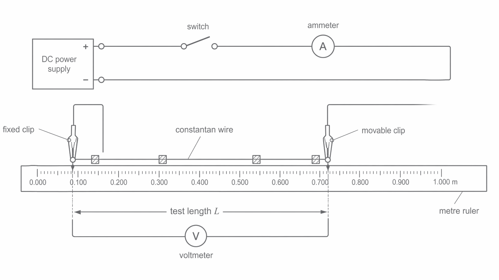
The first figure shows the full resistivity practical setup; notice that the ammeter is in series, the wire is stretched along the metre ruler, and the voltmeter is connected only across the measured section between the crocodile clips.
[DIAGRAM: asset_name: RP 05 - Determination of Resistivity of a Wire - Diagram 1; asset_slug: RP 05 - Determination of Resistivity of a Wire - Diagram 1; recommended_method: retained_png; description: Series circuit with a DC power supply, switch, and ammeter connected to a straight constantan wire taped along a metre ruler. One crocodile clip is fixed near the 0.000 m mark and the second clip is moved to set the test length L. A voltmeter is connected in parallel across the two clips only, so it measures the pd across the chosen length of wire and not across the whole circuit.]
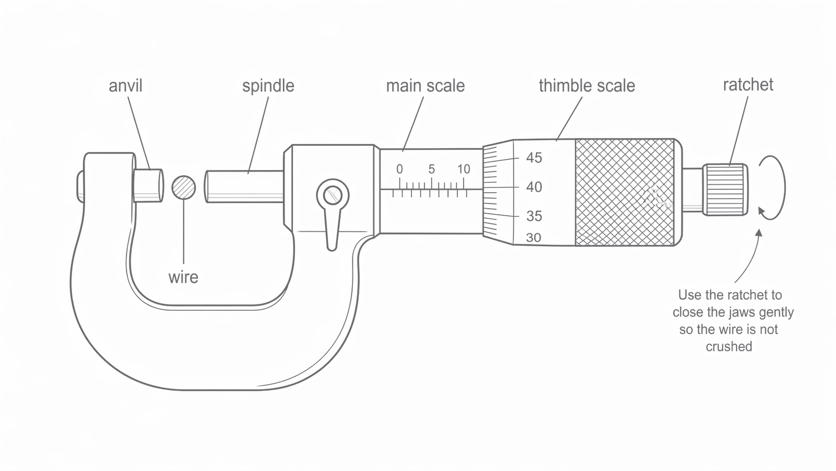
The second figure zooms in on the micrometer reading technique; notice the wire held lightly between the anvil and spindle and the ratchet being used to close the jaws gently without crushing the wire.
[DIAGRAM: asset_name: RP 05 - Determination of Resistivity of a Wire - Diagram 2; asset_slug: RP 05 - Determination of Resistivity of a Wire - Diagram 2; recommended_method: retained_png; description: Micrometer screw gauge measuring the diameter of the wire. Label the anvil, spindle, ratchet, main scale, thimble scale, and the wire between the jaws. Show that the ratchet is used to close the jaws gently so the wire is not crushed.]
Step-by-step method
-
Check the micrometer zero. Close the jaws gently with the ratchet and record any zero error before taking measurements.
-
Measure the wire diameter. Take several readings at different positions along the wire, and rotate the wire at each point to check it is close to circular. Use the ratchet each time and calculate the mean diameter .
-
Tape the wire straight along the metre ruler and build the circuit with the ammeter in series and the voltmeter across the chosen test length only.
-
Set the crocodile clips 0.100 m apart, close the switch briefly, record and , then open the switch and calculate .
-
Move one clip to new lengths such as 0.200 m, 0.300 m, up to 0.800 m. Adjust the supply if needed to keep the current moderate, and switch off between readings to limit heating.
-
Repeat the set of readings and calculate the mean resistance for each length.
-
Plot mean against , find the gradient, calculate , and then obtain the resistivity from .
The highest-value practical details are easy to memorise: keep the wire straight, use the ratchet on the micrometer, put the voltmeter across the measured section only, and disconnect the circuit between readings so the wire does not warm up significantly.
Part 3 — Variables, Controls, and Experimental Design
| Variable type | Description |
|---|---|
| Independent variable | Length of the wire between the crocodile clips, varied from 0.100 m to 0.800 m in 0.100 m steps |
| Dependent variable | Resistance , calculated from ammeter (resolution 0.01 A) and voltmeter (resolution 0.01 V) readings |
| Control 1 — Wire material | Use the same constantan wire throughout; different alloys have different resistivities |
| Control 2 — Wire diameter | Use the same continuous piece of wire; do not swap sections. Diameter is measured but must remain constant |
| Control 3 — Temperature | Switch off between readings and keep current low (~0.5 A) to prevent Joule heating changing the wire's resistance |
| Control 4 — Contact points | Ensure crocodile clips make firm, clean contact at each length; loose clips add variable contact resistance |
| Control 5 — Circuit components | Keep the same ammeter, voltmeter, and leads throughout to avoid introducing different systematic offsets |
The key to this practical is understanding which variables truly matter. Length and diameter are the geometric variables; temperature is the physical condition that must stay constant for Ohm's law to apply.
Repeats and range
Take at least two full sets of readings and calculate the mean at each length. Seven or more different lengths across the range 0.100–0.800 m provide enough data points to draw a reliable line of best fit and identify any anomalous results. A wide range is essential: if you only measured from 0.5 to 0.8 m, you would have insufficient spread to determine whether the line genuinely passes through the origin.
Part 4 — Expected Results, Graphs, and Interpretation
Sample results table
For a school setup using about 0.25 mm diameter constantan and keeping the current close to 0.50 A, a representative set of readings is:
| Length / m | Voltage / V | Current / A | Resistance / |
|---|---|---|---|
| 0.100 | 0.50 | 0.50 | 1.00 |
| 0.200 | 1.00 | 0.50 | 2.00 |
| 0.300 | 1.50 | 0.50 | 3.00 |
| 0.400 | 2.00 | 0.50 | 4.00 |
| 0.500 | 2.50 | 0.50 | 5.00 |
| 0.600 | 2.99 | 0.50 | 5.98 |
| 0.700 | 3.49 | 0.50 | 6.98 |
| 0.800 | 3.99 | 0.50 | 7.98 |
These values are close to what you expect from for constantan, while staying within the 0-1 A ammeter range described earlier.
The graph
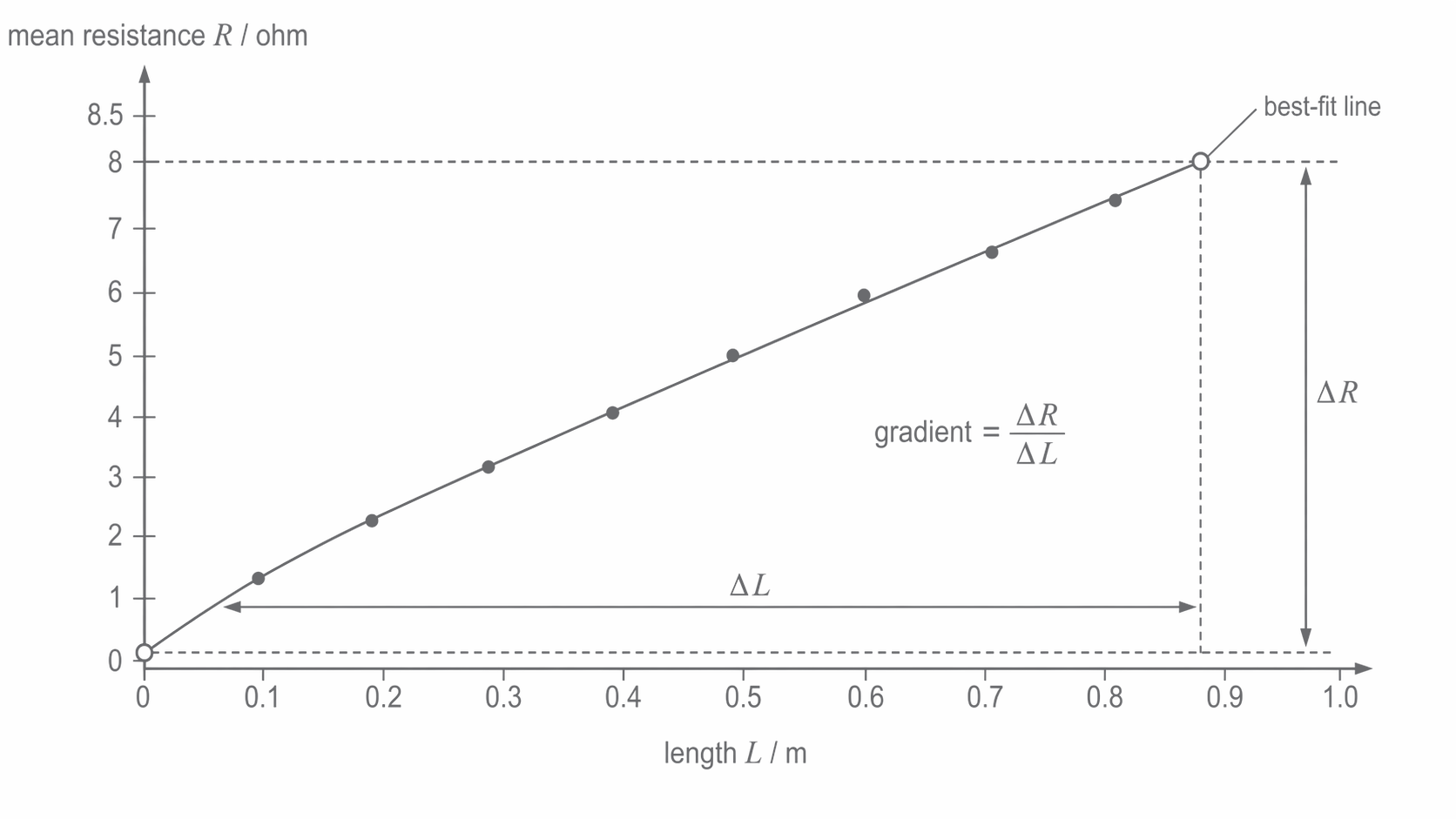
The figure below shows the expected resistance-length graph; notice the near-origin straight-line trend and that the gradient is taken from two widely separated points on the best-fit line rather than from raw data points.
[DIAGRAM: asset_name: RP 05 - Determination of Resistivity of a Wire - Diagram 3; asset_slug: RP 05 - Determination of Resistivity of a Wire - Diagram 3; recommended_method: retained_png; description: Graph of mean resistance / (y-axis, scale 0 to 8.5) against length / m (x-axis, scale 0 to 1.0). Eight data points rising in an approximately straight line from the origin. A best-fit straight line is drawn through the points, passing through or very close to the origin. The gradient is labelled as . Mark two widely separated points on the best-fit line (not data points) used to calculate the gradient.]
What to look for
The graph should be a straight line through the origin. This confirms the linear relationship — resistance is directly proportional to length when the cross-section and material are constant.
The gradient of this line equals . A steeper gradient means either higher resistivity or smaller cross-sectional area (thinner wire). For a 0.25 mm constantan wire, the gradient should be about .
If the best-fit line has a positive y-intercept rather than passing through the origin, this indicates a systematic error — most likely contact resistance at the crocodile clips, which adds a constant offset to every resistance measurement. A negative y-intercept could indicate a zero error on the metre ruler or that the clips were not placed exactly where you read the ruler.
Resistivity measurements are fundamental in materials science and the electronics industry. Semiconductor manufacturers measure the resistivity of silicon wafers using a four-point probe technique (an extension of the principle used here) to verify that doping levels are correct before fabricating microchips. A wafer with the wrong resistivity would produce transistors with incorrect switching thresholds, rendering an entire batch worthless.
If a data point falls noticeably off the line, it is anomalous. Common causes include a crocodile clip not making firm contact (giving a falsely high resistance) or the wire being kinked at that length (making the effective length different from the measured length). Anomalous points should be repeated and, if confirmed as outliers, excluded from the best-fit line.
Part 5 — Worked Example with Full Calculation
Let us work through the complete analysis using the representative 0.25 mm constantan data from Part 4.
Step 1 — Calculate the cross-sectional area
The measured mean diameter from the micrometer readings is:
The cross-sectional area is:
Step 2 — Calculate resistance at each length
Using for each pair of readings:
| / m | / V | / A | / |
|---|---|---|---|
| 0.100 | 0.50 | 0.50 | 1.00 |
| 0.200 | 1.00 | 0.50 | 2.00 |
| 0.300 | 1.50 | 0.50 | 3.00 |
| 0.400 | 2.00 | 0.50 | 4.00 |
| 0.500 | 2.50 | 0.50 | 5.00 |
| 0.600 | 2.99 | 0.50 | 5.98 |
| 0.700 | 3.49 | 0.50 | 6.98 |
| 0.800 | 3.99 | 0.50 | 7.98 |
Step 3 — Determine the gradient from the graph
Plot on the y-axis against on the x-axis. Draw the best-fit straight line. To calculate the gradient, choose two points on the line (not data points) that are far apart — for example:
- Point 1: ,
- Point 2: ,
Step 4 — Calculate resistivity
Step 5 — Compare with accepted value
The accepted resistivity of constantan is .
Our calculated value is essentially identical, so this dataset is a good example of the expected straight-line behaviour. In real school data there is usually a little more scatter, but the same gradient method is used.
The entire practical boils down to one equation: . The graph eliminates the need to trust any single measurement, and the gradient is immune to constant systematic offsets like contact resistance. The diameter measurement is the weakest link — its percentage uncertainty is doubled when calculating , so careful micrometer technique is by far the most important skill in this practical.
That summary is exactly why AQA likes mixed questions on this practical. You are often expected to combine a graph gradient with separate micrometer data, so the skill is joining the method and the graph logic into one chain rather than treating them as separate tasks.
Part 6 — Uncertainty and Error Analysis
Uncertainty analysis is where this practical becomes genuinely demanding — and where the most exam marks are concentrated. The critical insight is that the diameter measurement, despite appearing straightforward, dominates the total uncertainty because it is squared when calculating area.
Systematic errors in this practical
Zero error on the micrometer. If the micrometer does not read exactly 0.00 mm when the jaws are closed, every diameter measurement is shifted by the same amount. This error is always the same sign and magnitude, so it does not average out with repeats. Solution: Record the zero reading and subtract it from every measurement.
Contact resistance at crocodile clips. The imperfect metal-to-metal contact at the clips adds a small, roughly constant resistance to every measurement. This shifts the -vs- graph upward, producing a positive y-intercept. Solution: Use the gradient of the graph (unaffected by a constant offset) rather than individual calculations. Alternatively, use soldered connections or screw terminals.
Parallax error when reading the metre ruler. If you read the clip position from an angle rather than directly above, you consistently misread lengths. Solution: View the ruler perpendicularly from above.
Random errors in this practical
Fluctuating ammeter/voltmeter readings. Small variations in supply voltage or contact quality cause readings to scatter. Repeat measurements and averaging reduce this.
Positioning of crocodile clips. Each time you move a clip, you may not place it at exactly the intended position. This introduces scatter in the length measurement.
Variations in wire diameter. The wire is not perfectly uniform; the micrometer gives slightly different readings at different positions, introducing scatter in the calculated area.
Uncertainty calculations — worked through with numbers
Uncertainty in length ():
The metre ruler has mm graduations, so the resolution is 1 mm. Each clip position is read to . Since is the difference between two readings:
For : percentage uncertainty =
For : percentage uncertainty =
This is why longer lengths are more precise — the absolute uncertainty stays the same but becomes a smaller fraction of the measurement.
Uncertainty in diameter ():
The micrometer has a resolution of 0.01 mm. From our six readings (0.38, 0.37, 0.38, 0.39, 0.37, 0.38 mm in the earlier example), the spread is 0.39 − 0.37 = 0.02 mm. The uncertainty in the mean is estimated as:
For mean : percentage uncertainty =
Uncertainty in area ():
Since , and is squared:
This is the critical result. The diameter's percentage uncertainty is doubled because appears as . Even a modest uncertainty in becomes the dominant contribution to the overall uncertainty in . This is why the micrometer technique matters so much — and why examiners love to ask about it.
When asked which measurement contributes most to the uncertainty in resistivity, the safest answer is usually the diameter. That is because is squared in the area formula, so its percentage uncertainty is doubled. The metre ruler looks less precise, but its percentage uncertainty is typically much smaller than the percentage uncertainty in area.
Uncertainty in gradient:
Draw the steepest and shallowest acceptable lines through the data (lines that pass through the error bars of all points). Calculate the gradient of each.
- Best-fit gradient:
- Steepest gradient:
- Shallowest gradient:
Total uncertainty in resistivity ():
Since , and these are multiplied quantities:
For our calculated :
The accepted value of falls within this uncertainty range, confirming that our result is consistent with the true value.
Sources of error and improvements table
| Source of error | Type | Effect on result | Improvement |
|---|---|---|---|
| Micrometer zero error | Systematic | Shifts all diameter readings by a constant amount, causing to be consistently too large or too small, which directly scales | Record and subtract the zero error before every measurement session |
| Wire not perfectly straight (kinks) | Systematic | The true conducting length is longer than the measured ruler length, underestimating and therefore overestimating the gradient and | Gently straighten the wire before taping it to the ruler; avoid sharp bends |
| Contact resistance at crocodile clips | Systematic | Adds a constant resistance, producing a y-intercept on the graph; if individual values are used instead of the gradient, is overestimated | Use the graph gradient (immune to constant offsets); use soldered connections or 4 mm terminals |
| Heating of wire during measurement | Systematic (for metals, resistance increases) | Wire temperature rises, increasing resistance slightly, leading to overestimation of — though the effect is small for constantan | Switch off between readings; keep current around 0.5 A; take readings quickly |
| Parallax when reading the metre ruler | Random (if inconsistent) / Systematic (if consistently angled) | Introduces scatter or bias in length readings | Read the ruler from directly above, perpendicular to the scale |
| Variability in wire diameter | Random | Different micrometer readings at different positions introduce scatter in the calculated area | Take at least six measurements at different positions and orientations; use the mean |
Part 7 — Exam Context: How AQA Tests This Practical
Required Practical 5 brings together circuit construction, graphical analysis, uncertainty propagation, and the ability to adapt a known method to unfamiliar scenarios. These are the main ways the practical can be analysed.
Common question types
1. "Describe a method" (6-mark extended response). You are given the apparatus and asked to describe how to determine the resistivity of a wire. Full marks require: measuring diameter with micrometer (multiple readings, mean), setting up ammeter in series and voltmeter in parallel, varying length and recording and , calculating , plotting vs , using gradient × = . You must also mention switching off between readings to prevent heating.
2. Data analysis from given results. You are given a table of , , values and asked to calculate , plot the graph, determine the gradient, and find . Sometimes you are given the graph and asked to extract the gradient.
3. Evaluate a student's method. A hypothetical student has done the experiment; you must identify flaws, explain their effect, and suggest corrections.
4. Uncertainty calculations. Given raw measurements and their uncertainties, calculate the percentage uncertainty in the final answer. The doubling is almost always the focus.
5. Adapt the method. "How would you modify this experiment to investigate how resistivity depends on temperature?" or "Describe how to determine the resistivity of a material available only as a thin sheet."
Command words to expect
- State: a brief factual answer, no explanation needed.
- Explain: state the fact and give the reasoning/physics behind it.
- Calculate: show your working, give correct units, and use appropriate significant figures.
- Describe: a step-by-step account of what you would do — write as if instructing someone else.
- Evaluate: weigh up strengths and weaknesses, come to a conclusion.
- Suggest: apply your knowledge to an unfamiliar situation — there may be more than one valid answer.
Common student mistakes
- Using at a single point instead of the gradient. This fails to exploit the power of graphical analysis and is vulnerable to the y-intercept offset from contact resistance.
- Forgetting to double the percentage uncertainty in when calculating uncertainty in . The formula is ; the 2 in the power means you multiply the percentage uncertainty by 2.
- Confusing resistivity and resistance. Resistance is a property of a specific wire (); resistivity is a property of the material (). Examiners penalise incorrect units.
- Not converting mm to m. The micrometer reads in mm, but must be in m² and must be in . Forgetting the conversion by a factor of gives a final answer wrong by .
- Drawing the line of best fit through the first and last data points instead of through the overall trend. The best-fit line minimises the total distance from all points, not just the endpoints.
Four-point probe instruments used in semiconductor fabrication work on the same principle as this practical — measuring voltage and current to determine resistivity — but use four inline contacts to eliminate contact resistance entirely. The outer pair passes a known current; the inner pair measures the voltage drop. Since no current flows through the voltage contacts, contact resistance has no effect. This technique can measure the resistivity of silicon wafers to better than 1% accuracy.
Links to other specification points
This practical connects to several areas that could appear together in exam questions:
- 3.5.1.1 (Charge, current, and pd) — the definitions of , , and underpin every measurement.
- 3.5.1.3 (Resistivity) — the theory being tested; you must be able to recall and use .
- 3.5.1.2 (Current-voltage characteristics) — the ammeter-voltmeter method is the same technique used for I-V characteristics of components.
- 3.1.2 (Estimation) — you could be asked to estimate the resistance of a given wire from its dimensions.
- Uncertainty and error analysis (Practical Assessment) — percentage uncertainties, combining uncertainties, error bars and worst lines are examined in Paper 3 Section A.
One last exam point is worth keeping in mind before the final method question. Students often assume the metre ruler must dominate the uncertainty because it only reads to the nearest millimetre, but in practice the diameter is usually the bigger problem. That is because the percentage uncertainty in area is twice the percentage uncertainty in diameter, while the percentage uncertainty in a typical wire length is usually much smaller.
The final question tests the ability to write a complete method from scratch — this is the style that appears most frequently in Paper 3 and occasionally in the 6-mark questions on Papers 1 and 2.