RP03 - Determination of g by Free Fall
Every object near the Earth's surface accelerates downward at roughly the same rate, regardless of its mass, provided air resistance is negligible. This Required Practical asks you to measure that acceleration, , using a falling ball bearing, a ruler, and precision timing. The key challenge is the linearisation: the raw data do not give directly, so you rearrange the kinematics equation into a straight-line form and extract from a gradient. If you understand the derivation, the graphical analysis, and the uncertainty treatment, you can judge whether your final value is genuinely reliable.
Part 1: The Physics Behind the Practical
The experiment relies on the SUVAT equation for constant acceleration. When an object falls from rest (or from some initial velocity ), the displacement after time is given by the standard kinematics relation.
SUVAT displacement equation
Here is the vertical distance fallen between the two timing points, is the velocity of the ball bearing as it passes the first timing point, is the acceleration due to gravity (the quantity we want), and is the time to fall the distance .
Acceleration due to gravity, g
The acceleration experienced by any object in free fall near the Earth's surface, approximately , directed vertically downward. It is independent of the mass of the falling object when air resistance is negligible.
Why you cannot just use
If the ball were released from rest at exactly the point where timing begins, would be zero and you could plot against to get a straight line through the origin with gradient . In practice, timing begins at the upper light gate, but the ball has already been accelerating since it left the electromagnet above. That means , and there is an unknown initial velocity to deal with. We therefore need a linearisation that accounts for .
The vs linearisation (full derivation)
Starting from the displacement equation:
Divide both sides by (valid because for every data point):
Now multiply both sides by 2:
Linearised equation for free fall
Compare this with . If you plot on the -axis against on the -axis, you obtain a straight line where the gradient equals and the -intercept equals . This is the standard linearisation for the two-light-gate version of the practical.
Notice that the intercept is not needed for the final answer but its presence confirms that the ball had a non-zero velocity at the first timing point. If came out negative or implausibly large, that would signal a systematic error.
If you need to justify the graph choice, show the algebra explicitly: start from , divide by , multiply by 2, and then compare with .
Alternative linearisation: vs (release from rest)
If you use an electromagnet-and-trapdoor setup where timing starts at the moment of release (so ), the equation simplifies to . Plotting against gives a straight line through the origin with gradient . This is simpler, but it only works when timing begins exactly at release.
Part 2: Equipment, Setup, and Method
Equipment list
| Item | Purpose |
|---|---|
| Tall retort stand with heavy base or G-clamp | Supports apparatus vertically; must not topple |
| Electromagnet with low-voltage DC supply | Holds and cleanly releases the steel ball bearing |
| Steel ball bearing (small, dense) | The falling object; dense to minimise air resistance |
| Two light gates with bosses and clamps | Start and stop the electronic timer as the ball passes |
| Electronic timer or data logger (resolution ) | Measures the fall time between the two light gates |
| Metre ruler (mm graduations) | Measures the height between the light gates |
| 2 kg counterweight or G-clamp | Prevents the stand from toppling |
| Felt pad or sand tray | Cushions the ball bearing on landing; prevents bounce and damage |
| Plumb line | Ensures the ball bearing falls vertically through both light gates |
| Set square | Helps align the ruler vertically and reduce parallax |
Method A: Electromagnet with two light gates (recommended)
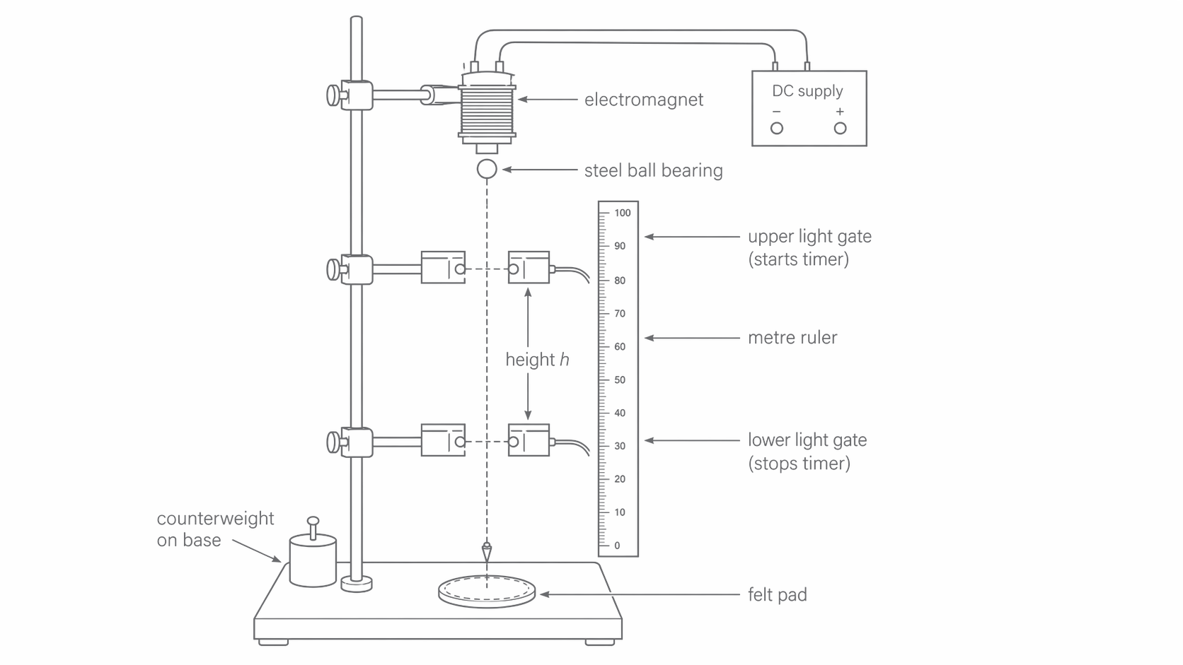
The schematic below shows the full apparatus layout; notice the fixed gap from the electromagnet to the upper light gate, the measured separation between the two light gates, and the plumb-line alignment through both gates.
[DIAGRAM: asset_name: RP 03 - Determination of g by a Free-Fall Method - Diagram 1; asset_slug: RP 03 - Determination of g by a Free-Fall Method - Diagram 1; recommended_method: retained_png; description: Apparatus setup. Tall retort stand clamped to bench. At the top, an electromagnet connected to a low-voltage DC supply holds a steel ball bearing. Below, two light gates are clamped to the stand, separated by a vertical distance . The upper light gate is connected to start the electronic timer; the lower light gate stops it. A metre ruler is clamped vertically alongside the light gates. At the base, a felt pad catches the ball. A plumb line hangs from the electromagnet to verify vertical alignment. Labels: electromagnet, DC supply, steel ball bearing, upper light gate (starts timer), lower light gate (stops timer), height , metre ruler, felt pad, counterweight on base.]
-
Clamp the retort stand securely to the bench using a G-clamp, or place a 2 kg counterweight on the base. The stand must not move during the experiment, because any wobble changes the fall path.
-
Mount the electromagnet at the top of the stand. Connect it to a low-voltage DC supply set at the manufacturer's recommended voltage.
-
Attach the two light gates to the stand using bosses. The upper light gate should be a fixed distance below the electromagnet (around 5 cm). This gap means the ball is already moving when it reaches the upper gate, giving the non-zero initial velocity discussed in Part 1.
-
Use a plumb line hung from the electromagnet to ensure the ball bearing will fall vertically through the centres of both light gates. Adjust the gates laterally until the plumb line passes through them. This step is essential because if the ball clips the edge of a gate, the timing will be inaccurate and the ball's trajectory will be deflected.
-
Connect the light gates to the electronic timer or data logger. The upper gate triggers the start; the lower gate triggers the stop.
-
Set the initial height between the upper and lower light gates, measured using the metre ruler. Clamp the ruler vertically alongside the gates and use a set square to read off the positions of the gate beam centres, reducing parallax error.
-
Switch on the electromagnet and hang the ball bearing from it. Reset the timer to zero.
-
Switch off the electromagnet to release the ball. The ball falls freely, triggering the upper gate (starting the timer) and the lower gate (stopping the timer). Record the time .
-
Repeat the drop three times at this height and calculate the mean time. Three repeats allows you to identify anomalies and reduces the effect of random timing errors.
-
Move the lower light gate up by 0.050 m to reduce to . Repeat the measurement process.
-
Continue reducing in steps of down to . Below this distance, the fall times become so short that percentage uncertainties in timing become unacceptably large.
-
Record all data in a table with columns: /m, /s, /s, /s, mean /s, / m s.
Method B: Electromagnet with trapdoor/impact switch (alternative)
In this arrangement, the timer is set to start when the release circuit is triggered and stop when the ball strikes a trapdoor or impact switch at the bottom. If the ball is released physically at the same instant the timer starts, then and the appropriate graph is against , giving a straight line through the origin with gradient .
The subtle point is the release delay. If the timer starts electrically when the electromagnet is switched off, but the ball remains stuck to the magnet for a short extra time because of residual magnetism, the recorded time is too long. That makes too large, the graph gradient too small, and the calculated value of too low. A mechanical release that starts timing at the instant the ball actually leaves the support deals with this more cleanly. Method A with two light gates usually avoids this problem and gives more precise timing.
AT k: using software and data logging well
AT k is not just "let the computer do the graph". A data logger or spreadsheet can record the light-gate times, calculate mean values, create a processed column such as or , and fit a straight line. You still need to choose the correct graph for the method used, check the units, inspect any outliers, and decide whether the intercept should be free or forced.
For Method A, plot against and keep the intercept free because it represents . For Method B, plot against ; only in that case should the line be expected to pass through the origin.
Precise measurement of local is critical in geophysics and mineral exploration. Gravimeters carried by aircraft and ships detect tiny variations in (of the order ) caused by differences in the density of underground rock. These surveys help locate oil, gas, and mineral deposits without drilling, saving enormous costs.
Part 3: Variables, Controls, and Experimental Design
Identifying variables clearly helps you describe the method properly and judge the quality of the data. Be specific about instruments and methods of control.
| Variable type | Description |
|---|---|
| Independent variable | Height between the two light gates, varied from down to in steps of |
| Dependent variable | Time for the ball to fall through the distance , measured by the electronic timer (resolution ) |
| Control 1 | Same ball bearing used throughout — a different size or mass would change air resistance effects |
| Control 2 | Distance from the electromagnet to the upper light gate kept constant — ensures is the same for every drop, which is essential for the linearisation to work |
| Control 3 | Electromagnet voltage kept constant — a weaker magnetic field might not hold the ball as firmly, causing it to slip slightly before release and changing |
| Control 4 | Ball released from the same position each time — repositioned against the same point on the electromagnet to ensure identical release conditions |
| Control 5 | Light gates not moved laterally between readings — only the lower gate's vertical position is changed, maintaining alignment |
Repeats
Each height should be repeated at least three times to allow calculation of a mean time. This reduces the effect of random variation in the ball's release (slight differences in how cleanly it detaches from the electromagnet).
Ensuring a suitable range
The range to gives at least six data points. For the most reliable gradient, your data points should span a wide portion of the graph. If a taller stand is available, starting at or higher is even better, because it extends the range and reduces the percentage uncertainty in height measurements.
Part 4: Expected Results, Graphs, and Interpretation
Sample results table
The table below shows realistic data for this experiment using the two-light-gate method. These are adapted from handbook sample results for the practical.
| / m | / s | / m s |
|---|---|---|
| 0.500 | 0.233 | 4.29 |
| 0.450 | 0.218 | 4.13 |
| 0.400 | 0.201 | 3.98 |
| 0.350 | 0.184 | 3.80 |
| 0.300 | 0.166 | 3.61 |
| 0.250 | 0.146 | 3.42 |
Notice that as decreases, decreases (shorter fall, less time) and also decreases because the average velocity over a shorter drop is lower.
The graph: against
The graph below shows the straight-line pattern to expect; notice that the gradient gives while the positive -intercept represents rather than zero.
[DIAGRAM: asset_name: RP 03 - Determination of g by a Free-Fall Method - Diagram 2; asset_slug: RP 03 - Determination of g by a Free-Fall Method - Diagram 2; recommended_method: retained_png; description: Graph with / s on the x-axis (range 0.14 to 0.24) and / m s on the y-axis (range 3.3 to 4.4). Six data points forming a straight line with a positive gradient. A best-fit line drawn through the points, extended to show the y-intercept at approximately (so ). The gradient is labelled as . Axes labelled with units. Title: "Graph of against for determination of ".]
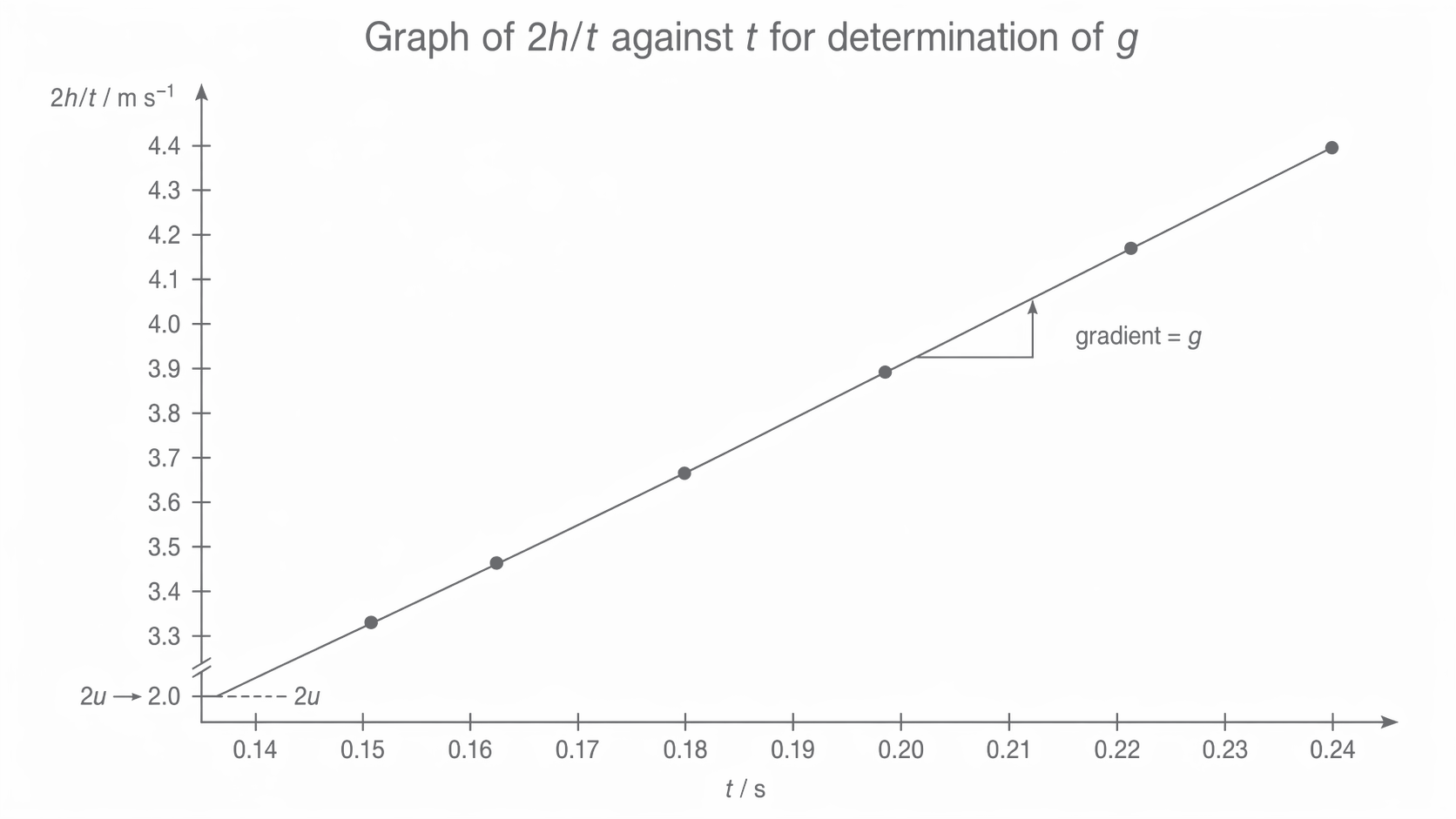
The graph should produce a straight line because the equation is linear in . Key features to note:
- Gradient = (the acceleration due to gravity). You should obtain a value close to .
- -intercept = , the initial velocity of the ball at the upper light gate multiplied by 2. This should be a positive value set by the fixed gap between the electromagnet and the upper light gate.
- The line should not pass through the origin because .
The physical interpretation of the positive gradient is straightforward: as the fall distance increases, the ball has more time to accelerate, so both and the average speed increase. The ratio increases linearly with because the acceleration is constant.
Linearisation
The process of rearranging a non-linear equation into the form so that a straight-line graph can be plotted. The gradient and/or intercept of the line then yield the quantity of interest. Linearisation is fundamental to A-level practical physics because it allows you to determine physical constants from graphical analysis rather than from a single measurement.
Alternative graph: against (for the trapdoor method)
If (trapdoor setup), plot on the -axis against on the -axis. This gives a straight line through the origin with gradient , so .
The handbook sample results for this method are:
| / m | / s | / s | / m s |
|---|---|---|---|
| 1.35 | 0.50 | 0.250 | 10.80 |
| 1.10 | 0.45 | 0.2025 | 10.86 |
| 0.85 | 0.40 | 0.160 | 10.63 |
| 0.65 | 0.35 | 0.1225 | 10.61 |
These values are systematically high (around on average versus ), so this particular dataset is not showing a release delay. A release delay from residual magnetism would make the measured times too long and would push the calculated value of lower, not higher. High values of instead suggest some combination of slightly underestimated times, slightly overestimated heights, or a timing interval that did not begin from true rest.
Part 5: Worked Example — Full Calculation
Here is the complete analysis using the sample data from Part 4 (two-light-gate method).
Step 1: Calculate processed quantities
The quantity has already been computed in the results table. For example, at and :
Step 2: Determine the gradient
Using two well-separated points on the best-fit line (not just data points, but points read from the line itself):
- Point 1 (from the line): ,
- Point 2 (from the line): ,
When reading the gradient from a graph, use two points that are far apart on the best-fit line rather than two original data points. A large gradient triangle reduces percentage reading error.
Step 3: State the result
Since gradient :
This is close to the accepted value of , which is what you would hope for from a well-aligned light-gate setup using a dense ball bearing and a sensible range of heights.
Step 4: Extract the -intercept
Extrapolating the best-fit line to :
Using the line equation: . Substituting one point:
So , giving . This is a plausible velocity for a ball that has already fallen a short distance before reaching the upper light gate.
Step 5: Percentage difference
A well-conducted experiment with good light gates and a tall stand should achieve a value within a few per cent of the accepted result. If your graph produced something much lower, that would point to significant error in the data or in the line of best fit rather than to the expected outcome of the method.
Part 6: Uncertainty and Error Analysis
Uncertainty analysis tells you whether your value of is convincing. You need to identify, classify, quantify, and improve the important sources of error.
Systematic errors in this practical
Systematic error
An error that shifts all measurements in the same direction by the same amount (or proportion). It cannot be reduced by repeating measurements. It is identified by comparing the final result with the accepted value.
Residual magnetism in the electromagnet: When the current is switched off, the core can retain magnetism for a short time. In the two-light-gate method, that delay happens before the timer starts, so by itself it does not change the measured fall time . In Method B, however, the timer may already be running while the ball is still attached, making every recorded time too long and the calculated value of too low.
Electronic switching delay: There can be a small delay in the release circuit or impact switch. This matters far more in Method B than in Method A, because Method A only times the motion between the two light gates.
Release not perfectly clean: If the ball does not detach from the electromagnet in exactly the same way every time, the initial speed at the upper light gate can vary slightly. In the two-light-gate method this mainly changes the intercept rather than the gradient, provided the gap to the upper gate is kept constant.
Random errors in this practical
Random error
An error that causes measurements to scatter unpredictably above and below the true value. It can be reduced by repeating measurements and calculating a mean.
Variation in ball release: The ball may not detach from the electromagnet identically every time, leading to slightly different initial velocities. This causes scatter in values at each height.
Parallax in reading the ruler: When measuring , if the observer's eye is not level with the light gate beam, the apparent position on the ruler shifts. This introduces random scatter in .
Electronic noise in the timer: The light gate and timer system may trigger slightly differently depending on exactly how the ball passes through the beam (e.g., if it spins or wobbles).
Worked uncertainty calculation
Let us work through the percentage uncertainty in from this experiment.
Uncertainty in :
The metre ruler has 1 mm graduations. You read two positions (upper and lower gate) each with an uncertainty of . The total uncertainty in is:
For the smallest height :
Uncertainty in :
The electronic timer has a resolution of . For the shortest time :
However, the dominant uncertainty in is more likely the random variation between repeats. If three readings at a given height are , , and , the range is and the uncertainty is:
Percentage uncertainty in :
Since is determined from the gradient of the vs graph, the uncertainty in is best found from the worst acceptable line (also called the steepest or shallowest line that still passes through the error bars of the data points).
If the best-fit gradient is and the worst acceptable line gives :
A well-conducted experiment should achieve a percentage uncertainty in of around 5-10%. If your uncertainty is larger, this suggests excessive scatter in your data.
To estimate the uncertainty in the gradient, draw a worst acceptable line: the steepest or shallowest straight line that still passes through the error bars. Compare its gradient with the best-fit gradient to judge the likely uncertainty in .
Sources of error and improvements
| Source of error | Type | Effect | Improvement |
|---|---|---|---|
| Residual magnetism holds the ball after current is switched off | Systematic | Ball is released slightly late; in Method B this makes the measured too long, so the calculated value of is too low | Use a mechanical release (e.g., hinged trapdoor) instead of an electromagnet, or use a non-magnetic ball with a cradle release |
| Electromagnetic braking (eddy currents in ball) | Systematic | Ball decelerates as it leaves the magnet, so initial part of fall is not free fall; is reduced | Increase the gap between the electromagnet and the upper light gate so the ball has time to reach true free-fall conditions before timing begins |
| Air resistance on the ball | Systematic | Opposes motion, so measured is slightly lower than true | Use a small, dense (steel) ball bearing to minimise the surface-area-to-mass ratio; drop over shorter distances to reduce the effect of terminal velocity approach |
| Parallax error when measuring | Random | Introduces scatter in values; could be in either direction | Clamp the ruler directly next to the light gates and use a set square to align eye level with the gate beam |
| Variation in release conditions | Random | Ball may not leave electromagnet identically each time, giving scatter in | Take at least 3 repeats at each height and use the mean; ensure the ball is placed in exactly the same position on the electromagnet before each drop |
| Ball not falling vertically through both gates | Random/Systematic | Effective fall distance differs from measured ; if ball clips gate it gives erroneous | Use a plumb line to align the gates vertically below the electromagnet; do trial runs before recording data |
In 4-6 mark evaluation questions, the best answers follow a clear chain: name a specific error, classify it if asked, say whether it makes or too large or too small, then explain how that changes the calculated value of . A vague phrase such as "human error" is not enough.
Part 7: Judging the Result
Once you have a value for , the next job is to decide whether the result is convincing. A strong conclusion does more than quote a number. It checks whether the graph is straight, whether the intercept is sensible, and whether the uncertainty is small enough for the accepted value to lie within the likely range of results.
A careful write-up should comment on four things:
- the plotted points lie close to a straight line, supporting the model
- the gradient gives a value of reasonably close to
- the intercept is positive and of a sensible size, showing that the ball was already moving at the upper light gate
- any remaining discrepancy is explained using specific sources of error rather than vague phrases such as "human error"
Common question-family traps
- In Method A, is the separation between the two light gates, not the full distance from the electromagnet to the lower gate.
- In Method A, the useful straight-line plot is against , not against .
- In Method A, a positive intercept is expected because it equals ; the line should not be forced through the origin.
- Repeats reduce random error, but they do not remove a systematic timing offset.
- An improvement only scores well if you link it to a named error and explain how it reduces that error.
The most reliable determination of comes from repeat timings, a wide range of heights, careful alignment, and a best-fit line on a graph of against .
This practical also links naturally to the rest of mechanics. The same constant acceleration appears again in free fall and projectile motion, and the same graph skills are used whenever you linearise data to extract a physical constant.