3.1.2 - Limitation of Physical Measurements
Every measurement in physics carries some degree of doubt. Understanding the nature, magnitude, and propagation of that doubt is essential: it determines how many significant figures you can justify, whether your result agrees with a theoretical prediction, and how you should design an experiment to minimise error. This lesson covers the types of error that arise in measurement, the vocabulary used to describe the quality of data, how to quantify uncertainty, how to combine uncertainties through calculations, and how to represent and extract uncertainties from graphs.
1. Types of Error
All experimental measurements are subject to error. It is useful to separate them into two categories.
Random Error
A random error causes measured values to fluctuate unpredictably above and below the true value, producing a spread of readings about the mean. Random errors affect the precision of a measurement.
Random errors arise from unpredictable variations in conditions or in the way an instrument is read. Examples include electronic noise in an electrical instrument, slight fluctuations in the thickness of a wire, and variability in human reaction time when using a stopwatch.
Reducing random errors:
- Take at least three repeat readings and calculate a mean; this also makes anomalies easier to spot and investigate.
- Use data loggers, computers, or cameras to remove human judgement from the timing or reading process and to enable smaller measurement intervals.
- Choose instruments with higher resolution (e.g. a micrometer at 0.01 mm rather than a ruler at 1 mm).
Systematic Error
A systematic error causes all readings to be shifted from the true value by the same amount (or the same proportion) in the same direction. Systematic errors affect the accuracy of a measurement.
Systematic errors originate in the apparatus itself or in a flaw in the experimental method. They are not reduced by repeating the measurement. Common examples include a balance that does not read zero when empty (a zero error) and reading a scale at an angle rather than at eye level (a parallax error).
Reducing systematic errors:
- Calibrate apparatus by measuring a known value (e.g. place a standard 1 kg mass on a balance); any discrepancy reveals the systematic offset.
- In radioactivity experiments, measure background radiation beforehand and subtract it from every reading.
- Read analogue scales at eye level, perpendicular to the scale, to eliminate parallax. Using a mirror behind the pointer and aligning the pointer with its image ensures a correct viewing angle.
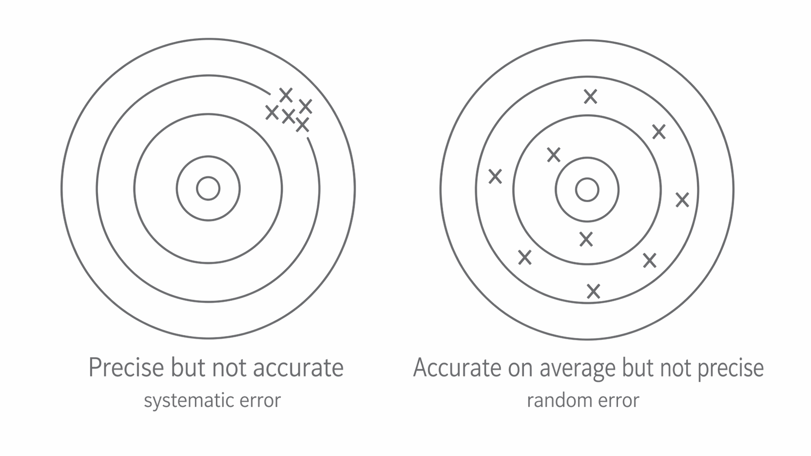
The target patterns below make the distinction visual: notice that systematic error can produce a tight cluster away from the true value, while random error gives a wider spread around the bullseye.
[DIAGRAM: asset_name: 1.2 - Limitation of Physical Measurements - Diagram 1; asset_slug: 1.2 - Limitation of Physical Measurements - Diagram 1; recommended_method: retained_png; description: Two target diagrams side by side. Left target shows shots clustered tightly together but away from the bullseye, labelled "Precise but not accurate — systematic error". Right target shows shots scattered around the bullseye, labelled "Accurate on average but not precise — random error".]
2. Describing the Quality of Measurements
It is important to distinguish five terms precisely. The cleanest way to remember them is to separate ideas about the spread of readings, the conditions of the repeat, and the quality of the instrument/result.
| Term | Meaning |
|---|---|
| Precision | Readings are closely clustered with little spread. Precision is mainly limited by random errors. |
| Repeatability | The same experimenter, using the same equipment and method, gets the same result on repeated trials. |
| Reproducibility | A different experimenter, or the same experimenter using different equipment or methods, gets the same result. |
| Resolution | The smallest change that produces a detectable change in the reading. |
| Accuracy | The result is close to the true or accepted value. |
Repeatability is tested within a single laboratory session. Reproducibility is a tougher test because it checks whether the result survives changes of person, equipment, or method. Resolution is a property of the instrument: a ruler marked every millimetre has a resolution of 1 mm, while a micrometer may resolve 0.01 mm. Higher resolution does not guarantee higher accuracy, but it limits how fine a measurement can be.
Note the important distinction: precision concerns the spread of repeated readings (random error), while accuracy concerns proximity to the true value (systematic error). A set of measurements can be precise without being accurate, and vice versa.
3. Quantifying Uncertainty
Uncertainty
The uncertainty of a measurement is the interval within which the true value can reasonably be expected to lie. It is expressed as a value an associated doubt, e.g. means the true temperature lies between 18 and 22 C.
Uncertainty can be expressed in three equivalent forms.
Absolute uncertainty — the doubt expressed as a fixed quantity in the same unit as the measurement:
Fractional uncertainty — the doubt expressed as a fraction of the measured value:
Percentage uncertainty — the doubt expressed as a percentage of the measured value:
Percentage Uncertainty
For the example above: , so the reading can be written as V, with fractional uncertainty or percentage uncertainty .
To reduce percentage (and fractional) uncertainty, measure larger quantities. For instance, timing 10 oscillations of a pendulum rather than 1 reduces the percentage uncertainty in the period by a factor of 10.
How to assign an uncertainty
The method depends on the type of measurement.
Single reading from an analogue instrument (e.g. a thermometer): the uncertainty is half the smallest division. If the smallest division is 1 C, the uncertainty is C.
A measurement involving two readings (e.g. a length measured with a ruler, where both the start and end positions are judged): each end contributes half the smallest division, so the total uncertainty is the smallest division. For a millimetre ruler, this is mm.
Digital instruments and quoted values: the uncertainty is the last significant digit unless stated otherwise. For example, a digital voltmeter reading 3.2 V has an uncertainty of V.
Repeated readings: the uncertainty is half the range of the readings.
Uncertainty from Repeated Readings
The result is expressed as: mean .
Significant figures and uncertainty
The number of significant figures quoted for a value should be consistent with its uncertainty. If the uncertainty in a length is m, then quoting the length as 1.2345 m implies false precision; it should be reported as 1.23 m. Uncertainties themselves are usually given to one significant figure (or at most two).
When CERN physicists reported the discovery of the Higgs boson in 2012, the mass was quoted as . The uncertainty communicated precisely how confident the collaboration was in the result and determined the number of significant figures justified in the reported mass.
4. Combining Uncertainties in Calculations
When measured quantities are combined in a formula, the uncertainties propagate into the final result. There are three standard cases to handle here. (Trigonometric and logarithmic combinations are not required.)
Case 1: Adding or subtracting quantities — add absolute uncertainties
If or , then:
Combining Uncertainties: Addition and Subtraction
where denotes the absolute uncertainty.
Worked example. A thermometer with an uncertainty of K shows a temperature drop from K to K.
Notice that subtraction can greatly increase the percentage uncertainty: here each reading has uncertainty, but the difference has uncertainty.
Case 2: Multiplying or dividing quantities — add percentage uncertainties
If or , then:
Combining Uncertainties: Multiplication and Division
Worked example. A force of N is applied to a mass of kg. Find the acceleration and its uncertainty.
Percentage uncertainty in :
Percentage uncertainty in :
Total percentage uncertainty in :
Convert back to absolute: of 13
Case 3: Raising to a power — multiply the percentage uncertainty by the power
If , then:
Combining Uncertainties: Powers
Worked example. The radius of a circle is cm. Find the area and its percentage uncertainty.
Percentage uncertainty in :
Since area , the power is 2:
Percentage uncertainty in :
When quantities are added or subtracted, add absolute uncertainties. When quantities are multiplied, divided, or raised to a power, work with percentage uncertainties: add them for products and quotients, and multiply by the power for exponents.
5. Representing and Extracting Uncertainties from Graphs
Error bars
Each data point on a graph can be given an error bar — a vertical line (and/or horizontal line) extending above and below (and/or left and right of) the point by an amount equal to the uncertainty in that quantity.
In the sketch below, notice that each vertical bar shows the uncertainty in a single y-value and that the best-fit line still passes through the range allowed by the data.
[DIAGRAM: asset_name: 1.2 - Limitation of Physical Measurements - Diagram 2; asset_slug: 1.2 - Limitation of Physical Measurements - Diagram 2; recommended_method: retained_png; description: A graph with data points plotted. Each point has a vertical error bar extending symmetrically above and below it. A straight line of best fit passes through all error bars. Labels indicate "error bar = +/- uncertainty in y" on one point.]
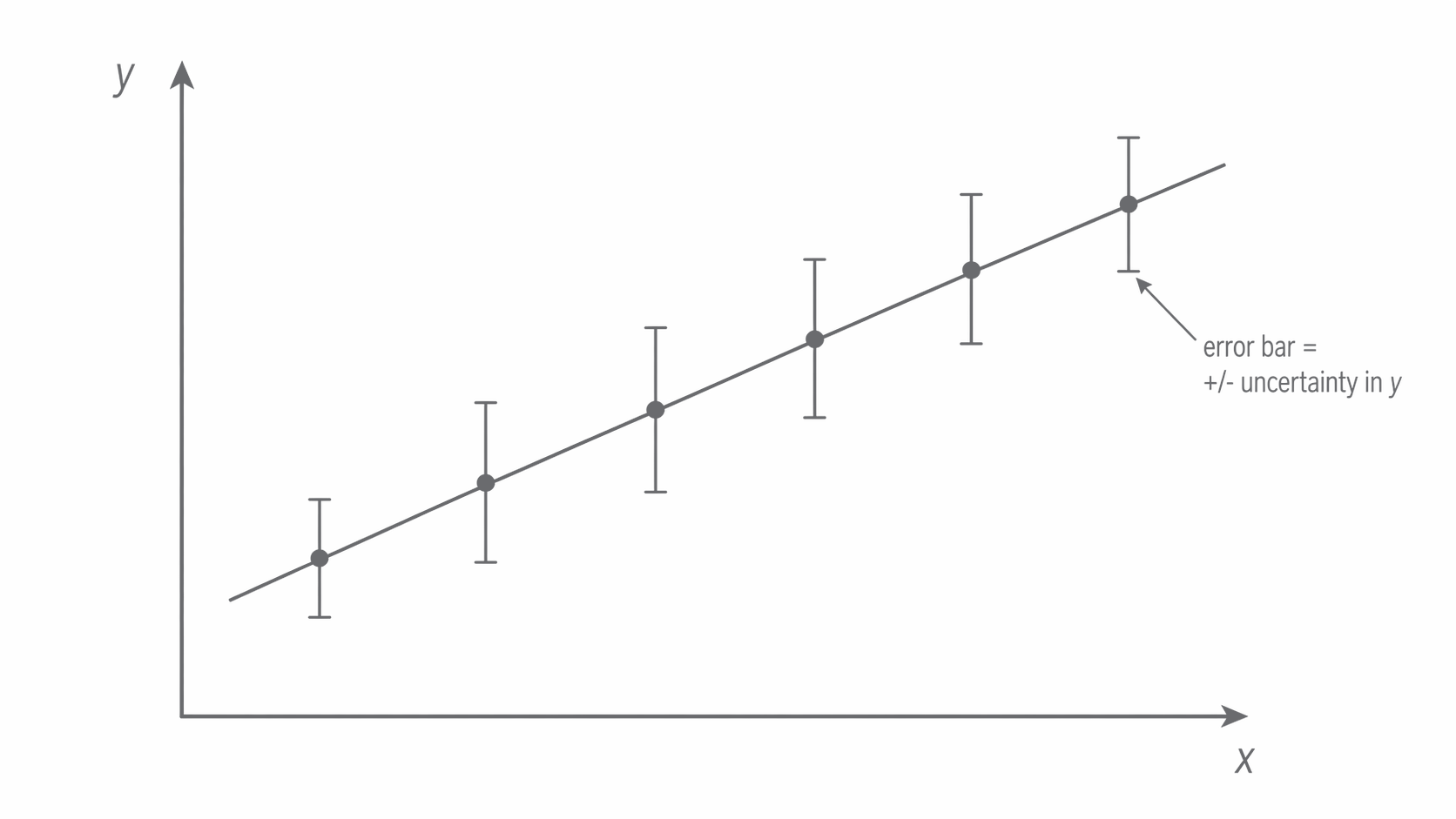
A line of best fit should follow the overall trend of the data and pass through as many error bars as is reasonably possible (excluding any anomalous points). If many error bars are missed, either the line choice is poor, there are anomalous points, or the uncertainties may have been underestimated.
Uncertainty in the gradient
To determine the uncertainty in the gradient of a straight-line graph:
- Draw the line of best fit through the data points.
- Draw the steepest acceptable line (the line of worst fit with the maximum gradient) that still passes through all error bars.
- Draw the shallowest acceptable line (minimum gradient) that still passes through all error bars.
- Calculate the gradient of each line.
Uncertainty in Gradient
Percentage Uncertainty in Gradient
An alternative convention uses both the maximum and minimum gradient lines:
Both methods are acceptable; the important thing is to be consistent.
Note that individual data points on a graph may or may not have associated error bars. When error bars are present, the worst-fit lines must pass through all error bars. When error bars are absent, draw the steepest and shallowest lines that could reasonably fit the data — these lines should still pass through or close to as many points as possible. The procedure for calculating the uncertainty in the gradient and intercept is the same in either case.
Uncertainty in the y-intercept
When the steepest and shallowest lines intercept the y-axis at different points, the uncertainty in the y-intercept is found in the same way:
The figure below shows what to compare: notice how the best-fit, steepest acceptable, and shallowest acceptable lines lead to different gradients and y-intercepts.
[DIAGRAM: asset_name: 1.2 - Limitation of Physical Measurements - Diagram 3; asset_slug: 1.2 - Limitation of Physical Measurements - Diagram 3; recommended_method: retained_png; description: A graph showing a line of best fit, a steepest line of worst fit, and a shallowest line of worst fit, all passing through the error bars. The different y-intercepts and gradients are labelled. Arrows indicate the difference between the best-fit gradient and the worst-fit gradient.]
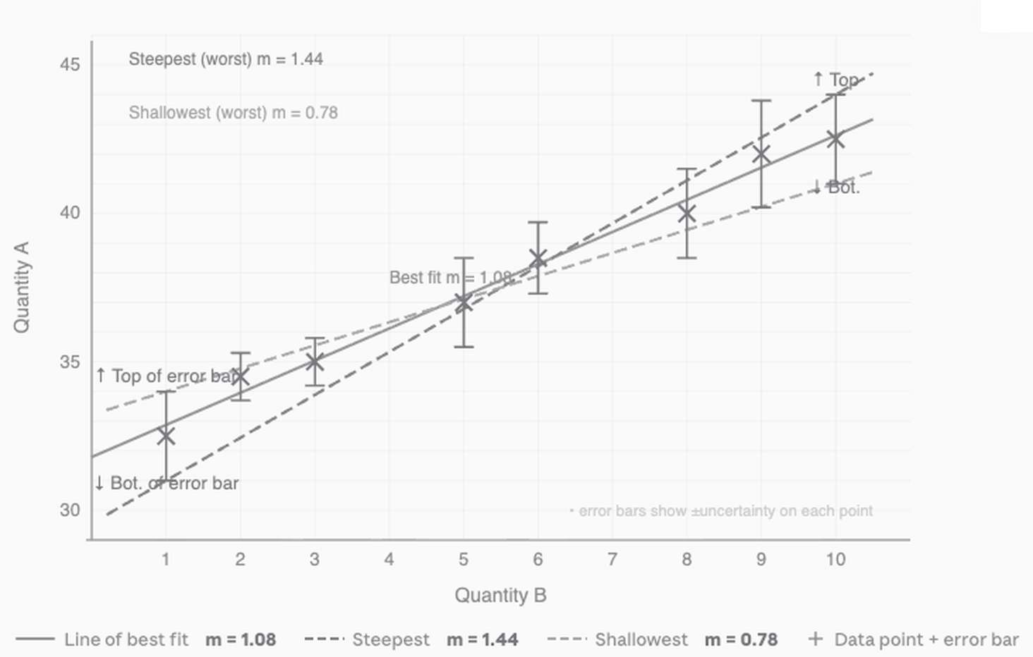
In a free-fall experiment to determine , students plot distance against time-squared . The gradient equals . By drawing best and worst fit lines through the error bars, the students can quote with an associated uncertainty and compare it to the accepted value of to evaluate the quality of their method.
6. Pulling It Together — Significant Figures and Good Practice
The number of significant figures in a final answer should reflect the size of the uncertainty, rather than just the raw number of digits entered into a calculator. In general:
- Quote uncertainties to 1 significant figure (occasionally 2 if the leading digit is 1).
- Quote the final value to the same number of decimal places as the uncertainty.
- Do not copy all the digits from a calculator display.
Identifying and reducing errors — a practical checklist:
| Error type | How to identify | How to reduce |
|---|---|---|
| Random | Spread of repeat readings about the mean | Take more repeats; use higher-resolution instruments; use data loggers |
| Systematic (zero error) | All readings offset by the same amount; non-zero reading when the instrument should read zero | Calibrate; check zero before use; subtract zero error |
| Systematic (parallax) | Reading depends on viewing angle | Read at eye level; use mirror scales |
| Systematic (background radiation) | Count rate higher than expected | Measure background and subtract |
This final problem pulls the measurement ideas together in a realistic analysis task.