Displacement, Speed, Velocity, and Acceleration

Before we can describe motion mathematically, we need precise definitions that distinguish between scalar and vector quantities.

Distance is the total length of path travelled, regardless of direction. It is a scalar.

Speed is the rate of change of distance — also a scalar.

Whereas speed tells us how fast an object is moving, velocity also tells us the direction. This distinction matters: a car driving in circles at constant speed has a constantly changing velocity.

Mathematically, velocity is calculated as the change in displacement divided by the time interval:

Where $\Delta s$ is the change in displacement and $\Delta t$ is the time interval.

A positive acceleration means the object is speeding up in the positive direction (or slowing down in the negative direction). A negative acceleration (often called deceleration in everyday language) means the velocity is becoming more negative — the object is either slowing down while moving in the positive direction or speeding up in the negative direction.

It is important to distinguish between instantaneous and average values:

• Average velocity is the total displacement divided by the total time: $\bar{v} = \frac{s}{t}$. It tells you nothing about what happened during the journey.
• Instantaneous velocity is the velocity at a specific moment. On a displacement–time graph, it equals the gradient of the tangent to the curve at that point.

The same distinction applies to speed. A car might have an average speed of $25\,\mathrm{m\,s^{-1}}$ over a journey while its instantaneous speed varies from $0$ to $30\,\mathrm{m\,s^{-1}}$.

Motion Graphs

Graphs are one of the most powerful tools in kinematics. The shape of a line, its gradient, and the area under it all carry physical meaning.

Displacement–time graphs

The gradient of a displacement–time graph gives the velocity.

• A straight line with a positive gradient indicates constant positive velocity (uniform motion).
• A straight line with a negative gradient indicates constant velocity in the negative direction.
• A horizontal line means the object is stationary ($v = 0$).
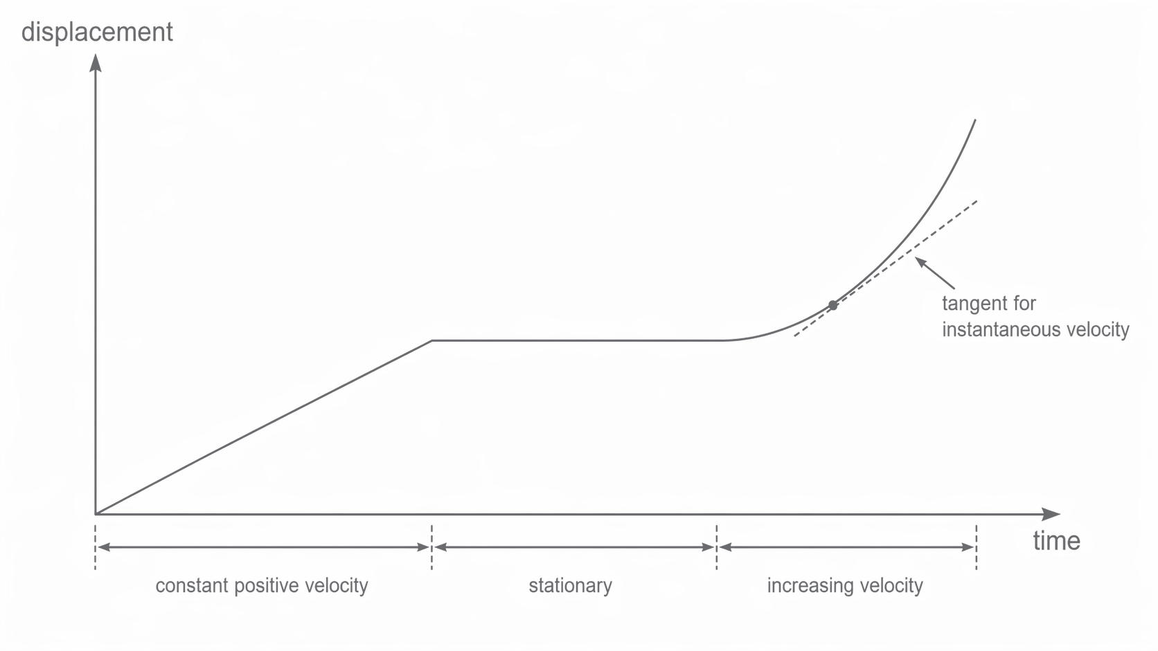
• A curve indicates changing velocity. The instantaneous velocity at any point is found by drawing a tangent and calculating its gradient.

The displacement-time graph below combines these cases, so notice how the gradient changes from positive, to zero, to increasingly steep as the object speeds up.

[DIAGRAM: asset_name: 4.1.3 - Motion Along a Straight Line - Diagram 1; asset_slug: 4.1.3 - Motion Along a Straight Line - Diagram 1; recommended_method: retained_png; description: A displacement–time graph showing three phases: (1) a straight line with positive gradient labelled "constant positive velocity", (2) a horizontal section labelled "stationary", and (3) a curve becoming steeper labelled "increasing velocity — draw tangent here to find instantaneous velocity".]

Velocity–time graphs

The gradient of a velocity–time graph gives the acceleration.

• A horizontal line means constant velocity (zero acceleration).
• A straight line with a positive gradient means uniform (constant) positive acceleration.
• A straight line with a negative gradient means uniform deceleration.
• A curve means the acceleration is changing (non-uniform acceleration). The instantaneous acceleration at any point is the gradient of the tangent at that point.

The area under a velocity–time graph gives the displacement.

• For uniform velocity, the area is a rectangle: $s = v \times t$.
• For uniform acceleration from $u$ to $v$, the area is a trapezium: $s = \frac{1}{2}(u + v)t$.
• For non-uniform motion, the total area can be estimated by counting squares or splitting the area into strips.

Acceleration–time graphs

The area under an acceleration–time graph gives the change in velocity.

For uniform acceleration, this area is a rectangle: $\Delta v = a \times t$. For non-uniform acceleration, the area must be estimated.

Deriving the SUVAT Equations

When acceleration is constant (uniform), four equations link five quantities: $s$ (displacement), $u$ (initial velocity), $v$ (final velocity), $a$ (acceleration), and $t$ (time). Each equation omits one of the five variables, so you always need to know three quantities to find a fourth.

Equation 1 — starting from the definition of acceleration:

Rearranging:

This is the most fundamental SUVAT equation. It says the final velocity equals the initial velocity plus the velocity gained through accelerating for time $t$.

Equation 2 — for uniform acceleration the average velocity is $\frac{u + v}{2}$, and displacement equals average velocity multiplied by time:

Equation 3 — substitute Equation 1 ($v = u + at$) into Equation 2:

This is particularly useful when you do not know the final velocity.

Equation 4 — eliminate $t$ by rearranging Equation 1 to give $t = \frac{v - u}{a}$ and substituting into Equation 2:

Rearranging:

This is the go-to equation when time is not given and not required.

Applying the SUVAT Equations

The key to solving SUVAT problems is a systematic approach:

1. Sketch the situation and define a positive direction.
2. List the known quantities — you need at least three of $s$, $u$, $v$, $a$, $t$.
3. Identify what you want to find.
4. Select the equation that contains only your three knowns and the unknown.
5. Substitute and solve. Keep proper signs throughout.

Here is a worked example following this method.

Worked Example: A driver of a vehicle travelling at $30\,\mathrm{m\,s^{-1}}$ on a motorway brakes sharply to a standstill in a distance of $100\,\mathrm{m}$. Calculate the deceleration.

Let positive be the direction of travel.

$u = 30\,\mathrm{m\,s^{-1}}$, $v = 0$, $s = 100\,\mathrm{m}$, $a = ?$

We need the equation without $t$: $v^2 = u^2 + 2as$

The negative sign confirms a deceleration (acceleration opposing the direction of motion).

When the direction of motion reverses during a problem, you may need to split the motion into stages. The link between stages is that the final velocity of one stage equals the initial velocity of the next.

Worked Example (two-stage): A ball is released from $0.85\,\mathrm{m}$ above a bed of sand and sinks $0.025\,\mathrm{m}$ into the sand. Find the deceleration in the sand.

Let positive be upwards.

Stage 1 (free fall): $u = 0$, $s = -0.85\,\mathrm{m}$, $a = -9.8\,\mathrm{m\,s^{-2}}$

$v^2 = 0 + 2 \times (-9.8) \times (-0.85) = 16.66$

$v = -4.08\,\mathrm{m\,s^{-1}}$ (negative, since moving downwards)

Stage 2 (in sand): $u = -4.08\,\mathrm{m\,s^{-1}}$, $v = 0$, $s = -0.025\,\mathrm{m}$

$0 = (-4.08)^2 + 2a \times (-0.025)$

$a = \frac{16.66}{0.050} = +333\,\mathrm{m\,s^{-2}}$

The positive sign indicates the acceleration is upwards — opposing the downward motion — confirming a deceleration of about $330\,\mathrm{m\,s^{-2}}$.

Free Fall and Acceleration Due to Gravity

Near the surface of the Earth, all objects in free fall experience the same acceleration regardless of their mass. This acceleration due to gravity is given the symbol $g$:

This value acts vertically downward. When using the SUVAT equations for vertical motion, adopt a sign convention: typically positive is upwards and negative is downwards, so $a = -g = -9.8\,\mathrm{m\,s^{-2}}$.

For an object dropped from rest ($u = 0$), the SUVAT equations simplify:

• $v = -gt$ (speed increases linearly with time)
• $s = -\frac{1}{2}gt^2$ (distance fallen increases with the square of time)
• $v^2 = -2gs$ (speed depends on distance fallen, not time)

Worked Example: A stone is dropped from a bridge $50\,\mathrm{m}$ above the water. Find (a) its speed just before hitting the water, (b) the time of fall.

Let positive be upwards. $u = 0$, $s = -50\,\mathrm{m}$, $a = -9.81\,\mathrm{m\,s^{-2}}$.

(a) $v^2 = u^2 + 2as = 0 + 2 \times (-9.81) \times (-50) = 981$

$v = -31.3\,\mathrm{m\,s^{-1}}$ (negative = downward), so speed $= 31.3\,\mathrm{m\,s^{-1}}$

(b) $v = u + at \Rightarrow -31.3 = 0 + (-9.81)t \Rightarrow t = 3.19\,\mathrm{s}$

For objects thrown upwards, the same equations apply. An object projected upwards at velocity $u$ decelerates at rate $g$, momentarily reaches $v = 0$ at its maximum height, then accelerates back down. The motion is symmetrical if air resistance is negligible: the speed at any given height is the same on the way up as on the way down.

At maximum height, $v = 0$, so using $v^2 = u^2 + 2as$:

The Bouncing Ball — Graphs and Analysis

The motion of a bouncing ball is a classic AQA example that combines free fall, velocity–time graphs, and the SUVAT equations. Understanding this scenario demonstrates mastery of the entire topic.

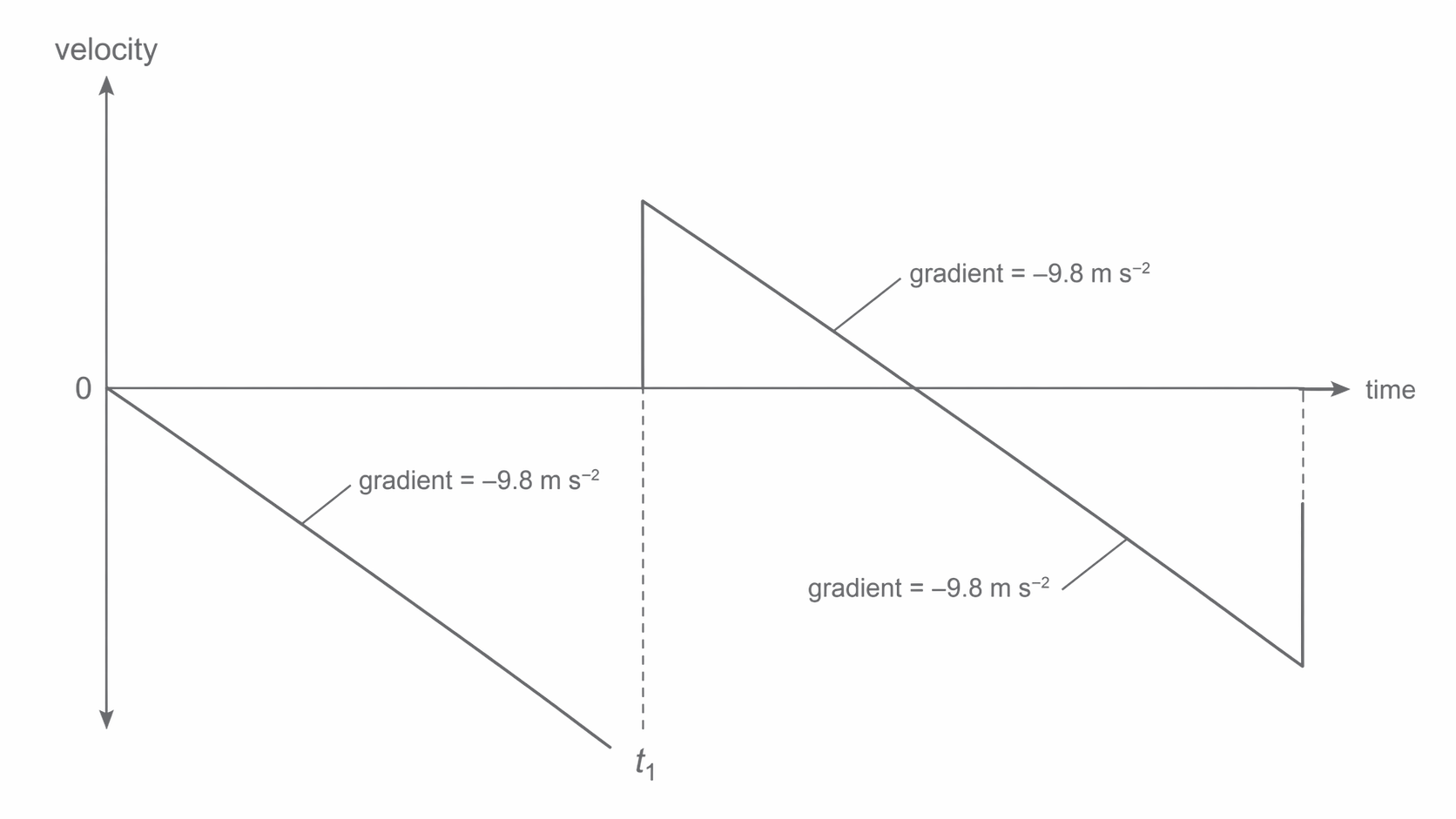
Consider a ball released from rest at height $h$ above a hard floor. It falls, bounces, rises to a lower height, falls again, and so on. The velocity-time graph below shows the constant downward gradient during each flight phase and the sudden jump in velocity when the ball rebounds from the floor.

[DIAGRAM: asset_name: 4.1.3 - Motion Along a Straight Line - Diagram 2; asset_slug: 4.1.3 - Motion Along a Straight Line - Diagram 2; recommended_method: retained_png; description: A velocity–time graph for a bouncing ball. The y-axis is velocity (positive upward). The graph shows a straight line starting at $v = 0$, sloping downward (becoming more negative) until the ball hits the floor at time $t_1$. At $t_1$ the velocity jumps instantaneously from a large negative value to a smaller positive value (the rebound). The line then slopes downward again at the same gradient ($-g$) to zero at maximum height, then continues downward to the next bounce. The gradient is constant at $-9.8\,\mathrm{m\,s^{-2}}$ throughout the flight phases.]

Key features of this graph:

• During free flight (between bounces), the gradient is constant at $-g = -9.8\,\mathrm{m\,s^{-2}}$, because only gravity acts.
• At each bounce, the velocity changes direction almost instantaneously. The speed just after the bounce is less than the speed just before, because kinetic energy is lost in the collision with the floor.
• At the top of each bounce, $v = 0$ momentarily.
• The area between the line and the time axis in each flight phase gives the displacement (height risen or fallen).

This graph perfectly illustrates the difference between speed and velocity: the speed is always positive (or zero), but the velocity is negative during descent and positive during ascent.