1. Density

This is one of the simplest but most useful quantities in materials physics, because it links a measurable mass to the amount of space a material occupies.

Here $\rho$ is density (kg m$^{-3}$), $m$ is mass (kg), and $V$ is volume (m$^{3}$). This equation can be rearranged to give $m = \rho V$ or $V = \frac{m}{\rho}$.

The SI unit of density is kg m$^{-3}$. A useful conversion: $1000\;\text{kg m}^{-3} = 1\;\text{g cm}^{-3}$, since $1\;\text{m}^3 = 10^6\;\text{cm}^3$.

Typical densities vary enormously between states of matter. Air has a density of about $1.2\;\text{kg m}^{-3}$, water $1000\;\text{kg m}^{-3}$, and lead $11\,300\;\text{kg m}^{-3}$. Gases are much less dense than liquids or solids because the average separation between molecules in a gas is far greater.

To measure density experimentally, measure the mass with a balance and the volume from dimensions or displacement. For this topic, the key point is using $\rho = \frac{m}{V}$ confidently with consistent SI units.

For example, a steel cylinder of diameter 12 mm and length 85 mm has radius $6.0 \times 10^{-3}\;\text{m}$, so its volume is $V = \pi r^2 h = \pi \times (6.0 \times 10^{-3})^2 \times 85 \times 10^{-3} = 9.6 \times 10^{-6}\;\text{m}^3$. Using $\rho = 7800\;\text{kg m}^{-3}$ then gives a mass of $m = \rho V = 7800 \times 9.6 \times 10^{-6} = 0.075\;\text{kg}$.

2. Hooke's Law and the Spring Constant

When a spring is stretched or compressed by an applied force, it extends or compresses. The relationship between the force and the extension was discovered by Robert Hooke.

Written mathematically, this proportional relationship is:

Here $F$ is the applied force (N), $k$ is the spring constant or stiffness constant (N m$^{-1}$), and $\Delta L$ is the extension from the natural (unstretched) length (m).

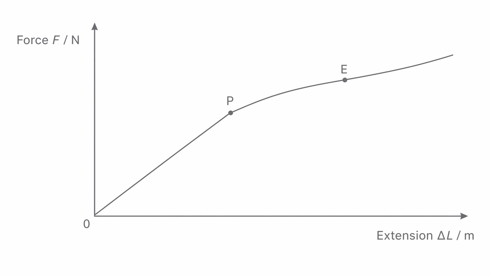
The spring constant $k$ is a measure of the stiffness of the spring --- the larger the value of $k$, the stiffer the spring. Graphically, a plot of $F$ against $\Delta L$ gives a straight line through the origin with gradient $k$, provided the spring obeys Hooke's law. In the graph below, notice that the straight-line Hooke's law region ends at $P$, while the elastic limit $E$ sits slightly beyond it.

[DIAGRAM: asset_name: 4.2.1 - Bulk Properties of Solids - Diagram 1; asset_slug: 4.2.1 - Bulk Properties of Solids - Diagram 1; recommended_method: retained_png; description: Force--extension graph for a spring. Straight line through the origin up to the limit of proportionality P. Beyond P the line curves. The elastic limit E is marked just beyond P. Axes: vertical = Force $F$ / N, horizontal = Extension $\Delta L$ / m.]

This tells you where the graph stops being a straight line. A closely related but slightly different idea is the elastic limit:

The limit of proportionality and the elastic limit are close together but not identical. The limit of proportionality marks where the graph departs from a straight line; the elastic limit is the point beyond which the material will not return to its original shape.

3. Tensile Stress and Tensile Strain

Force--extension graphs describe the behaviour of a specific object (a particular spring, wire, or strip). To compare the inherent mechanical properties of different materials regardless of their dimensions, we use stress and strain.

For a given force, a smaller cross-sectional area means a larger stress, which is why thin wires are easier to damage than thick cables made from the same material.

Here $\sigma$ (sigma) is stress (Pa), $F$ is the applied force (N), and $A$ is the cross-sectional area (m$^2$). For a wire of diameter $d$, the area is $A = \frac{\pi d^2}{4}$.

Because strain compares the extension with the starting length, it lets you compare samples of different sizes fairly.

Here $\varepsilon$ (epsilon) is strain (dimensionless), $\Delta L$ is the extension (m), and $L$ is the original length (m).

Stress and strain allow meaningful comparison between materials because they factor out the dimensions of the sample. A thin copper wire and a thick copper wire will have different force--extension graphs, but their stress--strain graphs will be identical (up to the same material limits) because stress and strain are properties of the material itself.

As a worked example, a wire of diameter $0.30\;\text{mm}$ has cross-sectional area $A = \frac{\pi d^2}{4} = \frac{\pi (3.0 \times 10^{-4})^2}{4} = 7.1 \times 10^{-8}\;\text{m}^2$. If it supports a tension of 60 N, the tensile stress is $\sigma = \frac{F}{A} = \frac{60}{7.1 \times 10^{-8}} = 8.5 \times 10^{8}\;\text{Pa}$.

4. Elastic Strain Energy and the Force--Extension Graph

When work is done stretching a material within its elastic limit, the energy is stored as elastic strain energy (also called elastic potential energy). Because the force varies linearly with extension (while Hooke's law holds), the work done is not simply $F \times \Delta L$ but rather the area under the force--extension graph.

For a spring or wire obeying Hooke's law, the stored energy comes from the triangular area under the force--extension graph.

For a material obeying Hooke's law, the force--extension graph is a straight line through the origin. The area under this line is a triangle, giving:

The first form, $E = \frac{1}{2} F \Delta L$, applies when you know the force at maximum extension. The second form, $E = \frac{1}{2} k (\Delta L)^2$, is obtained by substituting $F = k \Delta L$. Both forms give the energy in joules (J).

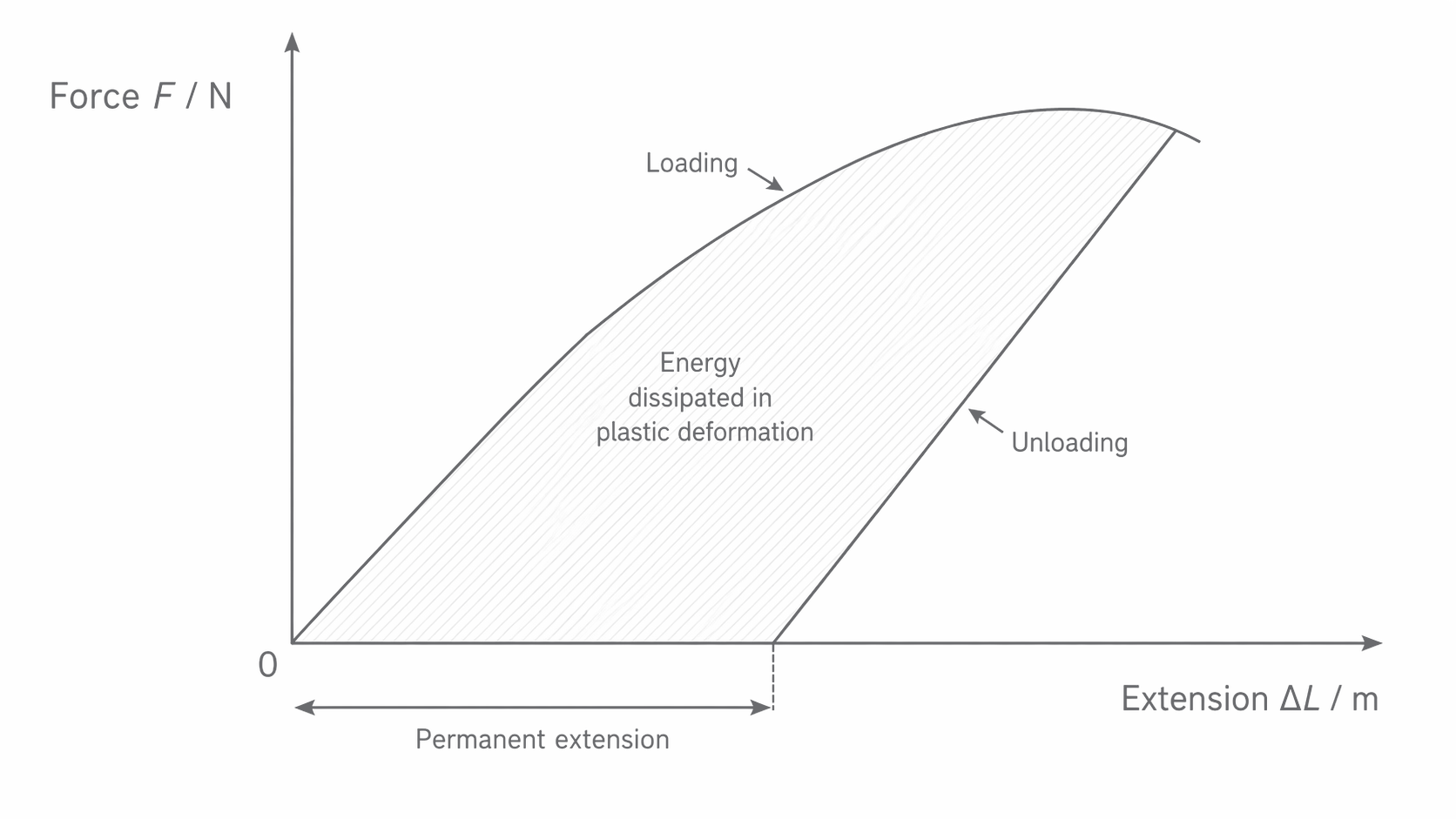
For a non-linear loading--unloading graph (for example, rubber), the area under the loading curve is the work done on the material during loading. The recoverable elastic strain energy is given by the area under the unloading curve. The area between the two curves is the energy dissipated as internal energy or heat.

Breaking stress is the stress at which a material fractures. On a stress--strain curve, it is the stress value at the fracture point.

Engineers must keep working stresses safely below the elastic limit and below the stress that would cause fracture.

The same equation is also useful in ordinary spring calculations, especially when you want to compare how the stored energy changes as the extension changes.

5. Plastic Behaviour, Brittle Fracture, and Ductile Materials

The force--extension graph of a material reveals much about its mechanical behaviour beyond the elastic limit.

Elastic behaviour: When a material is deformed within its elastic limit, it returns to its original shape when the force is removed. All the work done is stored as elastic strain energy and is fully recoverable.

Plastic behaviour: Beyond the elastic limit, the material undergoes permanent deformation. On a loading--unloading graph, the unloading line does not return to the origin. The unloading line is usually parallel to the initial straight-line elastic section, but it is offset --- the material has a permanent extension. The area between the loading and unloading curves represents the energy dissipated as heat during plastic deformation; this energy is used to move atoms to new permanent positions within the material. In the loading--unloading graph below, notice both the horizontal gap that shows the permanent extension and the shaded area that shows the energy dissipated during plastic deformation.

[DIAGRAM: asset_name: 4.2.1 - Bulk Properties of Solids - Diagram 2; asset_slug: 4.2.1 - Bulk Properties of Solids - Diagram 2; recommended_method: retained_png; description: Force--extension graph showing loading and unloading of a ductile material. Loading curve rises steeply then curves over. Unloading line is parallel to the initial straight section but offset to the right, not returning to the origin. The area between the curves is shaded and labelled "Energy dissipated in plastic deformation". The horizontal gap at zero force is labelled "Permanent extension".]

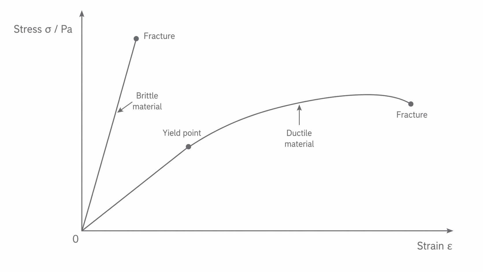
Brittle behaviour: A brittle material (e.g. glass, cast iron, ceramic) extends very little before fracturing. Its force--extension graph is nearly a straight line that ends abruptly at the point of fracture with no plastic region. Such materials obey Hooke's law right up to the breaking point.

Ductile behaviour: A ductile material (e.g. copper) can undergo a large amount of plastic deformation before fracturing. It can be drawn into a wire. On a stress--strain curve, a ductile material shows a large region between the elastic limit and fracture. In the comparison diagram below, notice how the brittle curve fractures soon after the linear region, while the ductile curve continues through a long plastic region before fracture.

[DIAGRAM: asset_name: 4.2.1 - Bulk Properties of Solids - Diagram 3; asset_slug: 4.2.1 - Bulk Properties of Solids - Diagram 3; recommended_method: retained_png; description: Stress--strain curves comparing a brittle material (steep straight line ending abruptly at fracture) and a ductile material (initial linear region, then a yield point, followed by a long plastic region before fracture). Axes: vertical = Stress $\sigma$ / Pa, horizontal = Strain $\varepsilon$.]

Interpreting stress--strain curves:

• The initial straight section shows that stress is proportional to strain.
• The elastic region is the part where the material returns to its original shape when unloaded.
• Beyond the elastic limit, the graph enters a plastic region, where permanent deformation occurs.
• A brittle material fractures with little plastic deformation, whereas a ductile material shows a much larger plastic region.
• The fracture point gives the breaking stress for that sample.

These graphs are useful because they summarise the whole story of a material from first loading through to permanent deformation and fracture.

6. Energy Conservation with Elastic Strain Energy

The specification requires quantitative and qualitative application of energy conservation to problems involving elastic strain energy.

Spring energy transformed to kinetic and gravitational potential energy: Consider a spring compressed and then released to launch an object vertically. It is safest to compare clearly defined stages rather than writing one blanket equality.

If the object's change in height while it is still in contact with the spring is negligible, the elastic strain energy initially stored becomes kinetic energy as the object leaves the spring:

After the object has left the spring, that kinetic energy is converted to gravitational potential energy as it rises:

For the whole motion from the compressed starting position to the highest point, you may write $\frac{1}{2} k (\Delta L)^2 = mg\Delta h$ provided $\Delta h$ is the total vertical rise from the starting position and resistive forces are negligible.

Similarly, when a mass on a vertical spring oscillates, energy continuously transfers between elastic strain energy (at maximum extension or compression), kinetic energy (as the mass passes through equilibrium), and gravitational potential energy (at the highest point). At every instant, the total mechanical energy is conserved (assuming no energy losses).

The specification asks students to appreciate energy conservation issues in the context of ethical transport design. This means understanding that:

• In a collision, kinetic energy must be transferred to other forms. The longer the deformation time and distance, the smaller the average force on occupants (from $F = \frac{\Delta p}{\Delta t}$).
• Plastic deformation in crumple zones absorbs energy permanently, preventing it from being transferred back to the passengers.
• Materials with appropriate breaking stresses and plastic behaviour are deliberately chosen for crumple zones.
• There are ethical considerations: safer vehicles may be heavier and consume more fuel, increasing environmental impact. Engineers must balance safety with sustainability.

For example, a spring of constant $150\;\text{N m}^{-1}$ compressed by $0.040\;\text{m}$ stores $\frac{1}{2}k(\Delta L)^2 = \frac{1}{2} \times 150 \times 0.040^2 = 0.12\;\text{J}$. If the spring launches a $0.012\;\text{kg}$ dart horizontally, or if any change in height during release is negligible, all of that energy becomes kinetic energy of the dart. Then $\frac{1}{2}mv^2 = 0.12$, so $v = \sqrt{\frac{2 \times 0.12}{0.012}} = 4.5\;\text{m s}^{-1}$.

Now consider how these ideas link together in an extended problem.

A complete explanation combines the energy calculation with the idea that plastic deformation prevents that energy being returned to the car.