3.6.1.2 - Simple Harmonic Motion
Simple harmonic motion (SHM) is one of the most important types of motion in physics. From the swing of a pendulum to the vibration of atoms in a crystal lattice, SHM underpins a vast range of physical phenomena. In this lesson you will learn the defining conditions of SHM, the key equations that describe displacement, velocity, and acceleration, and how to interpret the graphical relationships between these quantities.
1. What is Simple Harmonic Motion?
An oscillation occurs whenever an object moves repeatedly back and forth through an equilibrium position. The equilibrium position is the point at which the object would remain at rest if undisturbed. Not every oscillation qualifies as SHM; the motion must satisfy two strict conditions simultaneously.
Simple Harmonic Motion
Oscillating motion in which the acceleration of the object is directly proportional to its displacement from the equilibrium position and is always directed towards that equilibrium position (i.e., in the opposite direction to the displacement).
These two conditions can be expressed compactly as:
The negative sign is essential: it encodes the requirement that the acceleration always acts back towards equilibrium, opposing the displacement. Without this restoring nature, the motion would not be oscillatory.
Defining Equation of SHM
In this equation:
- is the acceleration of the object (m s),
- is the displacement from the equilibrium position (m),
- is the angular frequency of the oscillation (rad s), defined as , where is the time period and is the frequency.
The constant of proportionality is , which means that a shorter time period (faster oscillation) produces a larger acceleration for any given displacement.
Angular Frequency
The angular frequency is defined as , where is the time period and is the frequency. It is measured in rad s.
Some key terms used throughout this lesson are worth defining precisely here.
Amplitude
The amplitude of an oscillation is the maximum displacement of the oscillating object from its equilibrium position.
The amplitude tells you how far the object travels from its rest position. Closely related are two quantities that describe how quickly the oscillations repeat.
Time Period
The time period is the time taken for one complete cycle of oscillation. One full cycle returns the object to the same position, moving in the same direction.
The reciprocal of the time period gives the frequency of the oscillation.
Frequency
The frequency is the number of complete oscillations per unit time. It is measured in hertz (Hz), where 1 Hz = 1 cycle per second. It is related to the time period by .
The figure below shows the equilibrium position, an intermediate displacement, and both turning points; notice that amplitude is measured from the centre to an extreme while the restoring acceleration at the extremes points back towards equilibrium.
[DIAGRAM: asset_name: 6.1.2 - Simple Harmonic Motion - Diagram 1; asset_slug: 6.1.2 - Simple Harmonic Motion - Diagram 1; recommended_method: retained_png; description: An oscillating object shown on a horizontal line at three positions. The centre is labelled "equilibrium position, ". The left turning point is labelled "" and the right turning point "". A shorter arrow from the centre to an intermediate point is labelled "displacement ". A full arrow from the centre to one turning point is labelled "amplitude ". Arrows at both turning points point back towards the centre to show the restoring acceleration.]
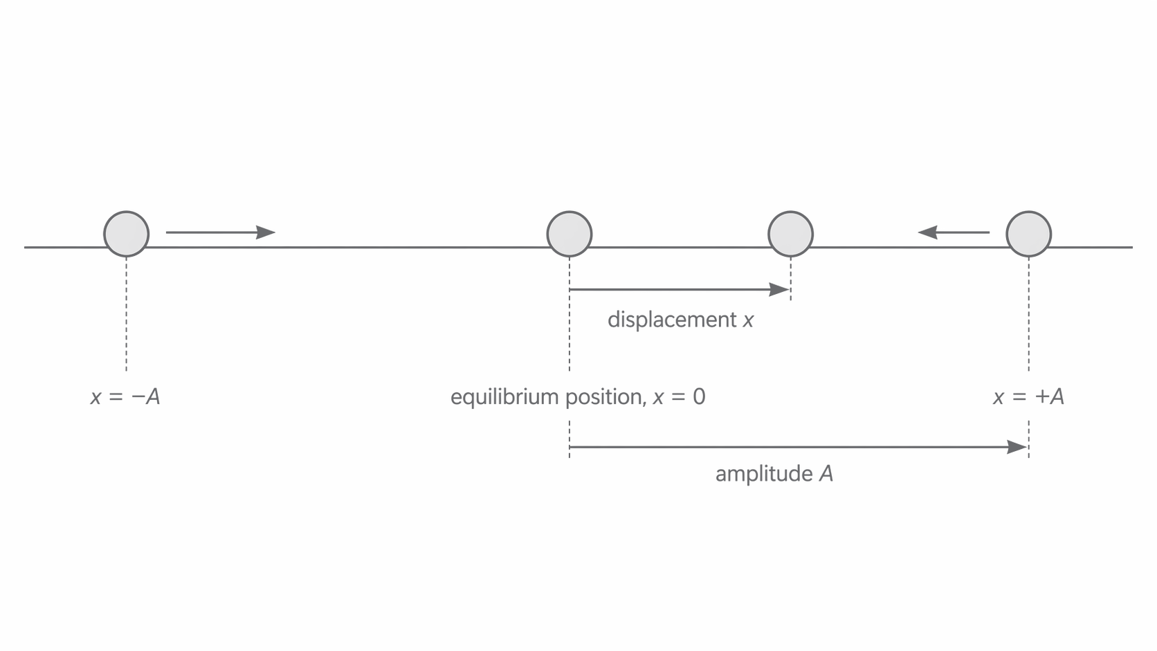
This diagram helps separate two ideas that students often merge. The displacement is the object's current signed distance from equilibrium, so it can be positive, negative, or zero. The amplitude is the largest value that ever reaches. Equilibrium is the midpoint of the motion, not one end of it.
Consider a simple pendulum: when displaced to one side and released, the restoring component of its weight always acts back towards the lowest point (the equilibrium). At maximum displacement (the amplitude), the acceleration is at its greatest magnitude because is at its maximum. At the equilibrium position (), the acceleration is zero.
2. Displacement as a Function of Time
The defining equation is a second-order differential equation. Its solution gives displacement as a sinusoidal function of time. If we choose to start timing () at the instant when the object is at maximum positive displacement (), the solution is:
Displacement–Time Equation
Here is the amplitude and must be calculated in radians (ensure your calculator is in radian mode).
This cosine form applies when the object starts at . If instead timing begins as the object passes through equilibrium moving in the positive direction, the displacement follows . Both are valid solutions; which one to use depends on the initial conditions of the problem.
The time period does not depend on the amplitude. Whether you pull a pendulum back by a small angle or a larger angle (within the SHM approximation), the period remains the same. This is a hallmark of SHM.
Worked Example: An object oscillates in SHM with amplitude 58 mm and time period 3.0 s. Find its displacement at s, given that it starts at maximum positive displacement.
Solution:
At s (which is ), the object has moved from 58 mm to 29 mm — it is returning towards equilibrium.
3. Velocity in SHM
Velocity in SHM can be expressed as a function of displacement using the equation:
Velocity–Displacement Equation
The sign indicates that for any given displacement (other than ), the object could be moving in either direction — towards or away from that point.
From this equation, several important results follow:
- At the equilibrium position (): . This is the maximum speed.
- At the extremes (): . The object is momentarily at rest before reversing direction.
Maximum Speed
This makes physical sense: the object is fastest as it passes through the centre and stationary at the turning points.
Earthquake-resistant building design relies on understanding SHM. During seismic activity, buildings oscillate laterally. Engineers model these oscillations using SHM principles to calculate the maximum velocity and acceleration experienced by the structure. By knowing , they can determine how quickly floors move at the equilibrium crossing, which directly informs the specification of damping systems to absorb kinetic energy and prevent structural failure.
Worked Example: A mass on a spring oscillates with amplitude 0.040 m and frequency 1.5 Hz. Calculate the maximum speed of the mass.
Solution:
4. Acceleration in SHM
From the defining equation , the magnitude of the acceleration is greatest when is greatest, that is, when the object is at maximum displacement ().
Maximum Acceleration
At the equilibrium position (), the acceleration is zero. This is the exact opposite of velocity: velocity is maximum where acceleration is zero, and acceleration is maximum where velocity is zero.
Worked Example: An object on a spring oscillates with time period 0.48 s and maximum acceleration 9.8 m s. Calculate (a) its frequency, and (b) its amplitude.
Solution:
(a) Hz Hz
(b) From :
5. Graphical Representations: Linking , , and with Time
One of the most important skills in SHM is understanding and interpreting displacement–time, velocity–time, and acceleration–time graphs, and appreciating how they are connected through calculus (differentiation).
Displacement–time graph ( vs ): Since , the graph is a cosine curve oscillating between and with period .
The figure below stacks the three time graphs on one shared axis; notice how the dashed guide lines connect turning points, zero crossings, and the phase shifts between , , and .
[DIAGRAM: asset_name: 6.1.2 - Simple Harmonic Motion - Diagram 2; asset_slug: 6.1.2 - Simple Harmonic Motion - Diagram 2; recommended_method: retained_png; description: Three vertically stacked graphs sharing the same time axis. Top graph: vs , a cosine curve with amplitude , labelled maxima at and minima at . Middle graph: vs , a negative sine curve with amplitude . Bottom graph: vs , a negative cosine curve with amplitude . Vertical dashed lines at , , , , and connect corresponding points across all three graphs.]
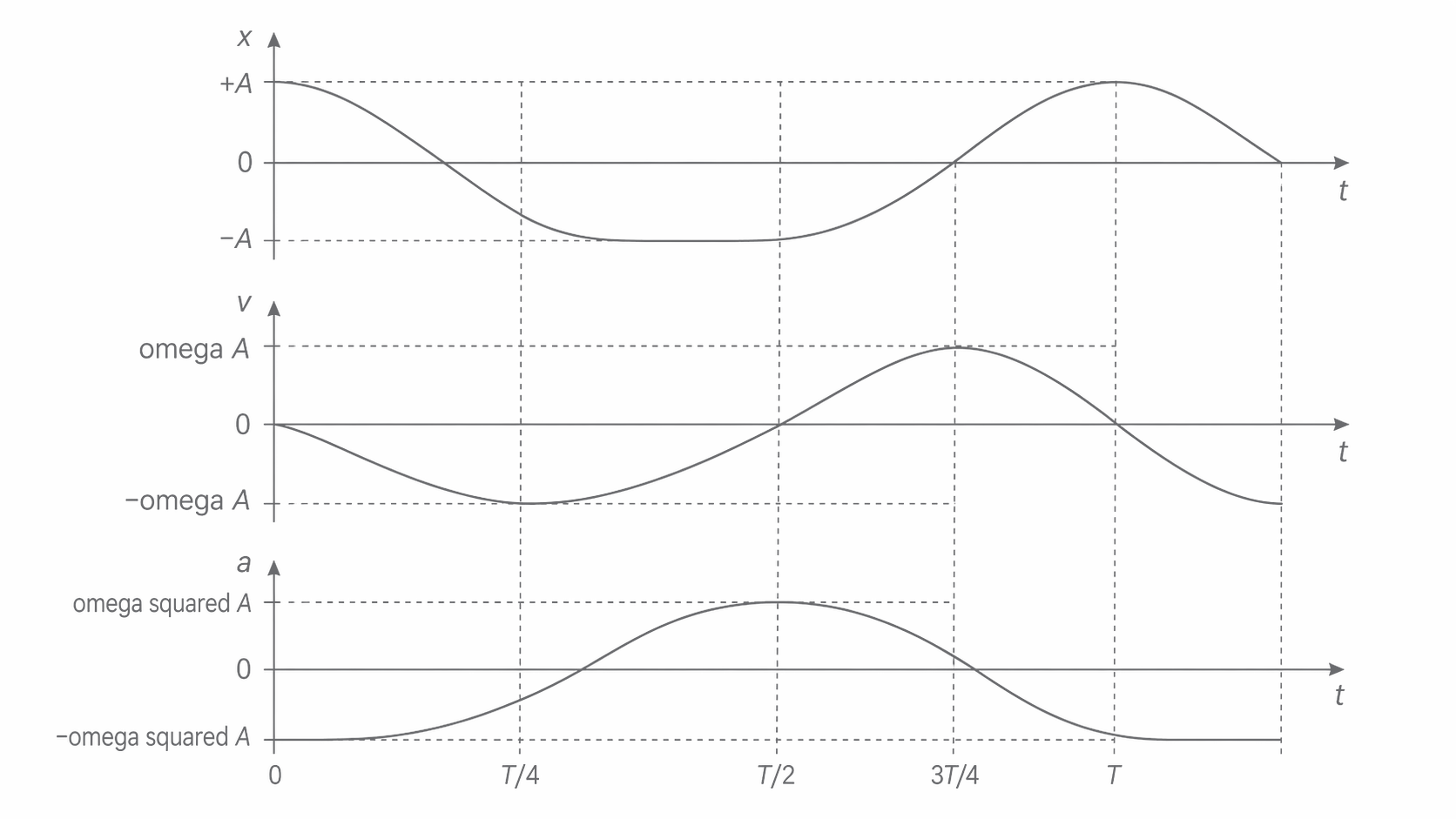
Velocity–time graph ( vs ): Velocity is the gradient (derivative) of the displacement–time graph. If , then . This is a negative sine curve:
- When displacement is at a maximum (), the gradient of the – graph is zero, so .
- When displacement is zero (object passing through equilibrium), the gradient is steepest, giving .
The velocity–time graph leads the displacement–time graph by a quarter of a cycle ( radians or 90°). More precisely, velocity reaches its maximum value a quarter period before displacement reaches its maximum.
Acceleration–time graph ( vs ): Acceleration is the gradient of the velocity–time graph. Differentiating again: , which confirms the defining equation. The acceleration–time graph is an inverted cosine curve:
- Maximum positive acceleration occurs at maximum negative displacement.
- Maximum negative acceleration occurs at maximum positive displacement.
The acceleration is exactly in antiphase with the displacement — a phase difference of radians (180°).
The velocity–time graph is the gradient of the displacement–time graph, and the acceleration–time graph is the gradient of the velocity–time graph. Acceleration is always in antiphase ( rad) with displacement; velocity leads displacement by rad.
These relationships are summarised in the table below:
| Quantity | At (max displacement) | At (equilibrium) | At (max negative displacement) |
|---|---|---|---|
| Displacement | (max) | 0 | (min) |
| Velocity | 0 | (max magnitude) | 0 |
| Acceleration | (max magnitude, negative) | 0 | (max magnitude, positive) |
6. The Connection Between Circular Motion and SHM
The mathematics of SHM is intimately connected to uniform circular motion. Consider a point P moving at constant speed around a circle of radius . If you project the position of P onto one axis (say the -axis), the projection oscillates back and forth between and — this projected motion is SHM.
The figure below shows the circular-motion model; notice how the horizontal projection of point P gives the SHM displacement while the angle controls where that projection falls.
[DIAGRAM: asset_name: 6.1.2 - Simple Harmonic Motion - Diagram 3; asset_slug: 6.1.2 - Simple Harmonic Motion - Diagram 3; recommended_method: retained_png; description: A circle of radius centred at the origin. A point P is shown on the circle at angle from the positive -axis. A vertical dashed line drops from P to the -axis, showing the projection . The angular velocity is labelled along the arc.]
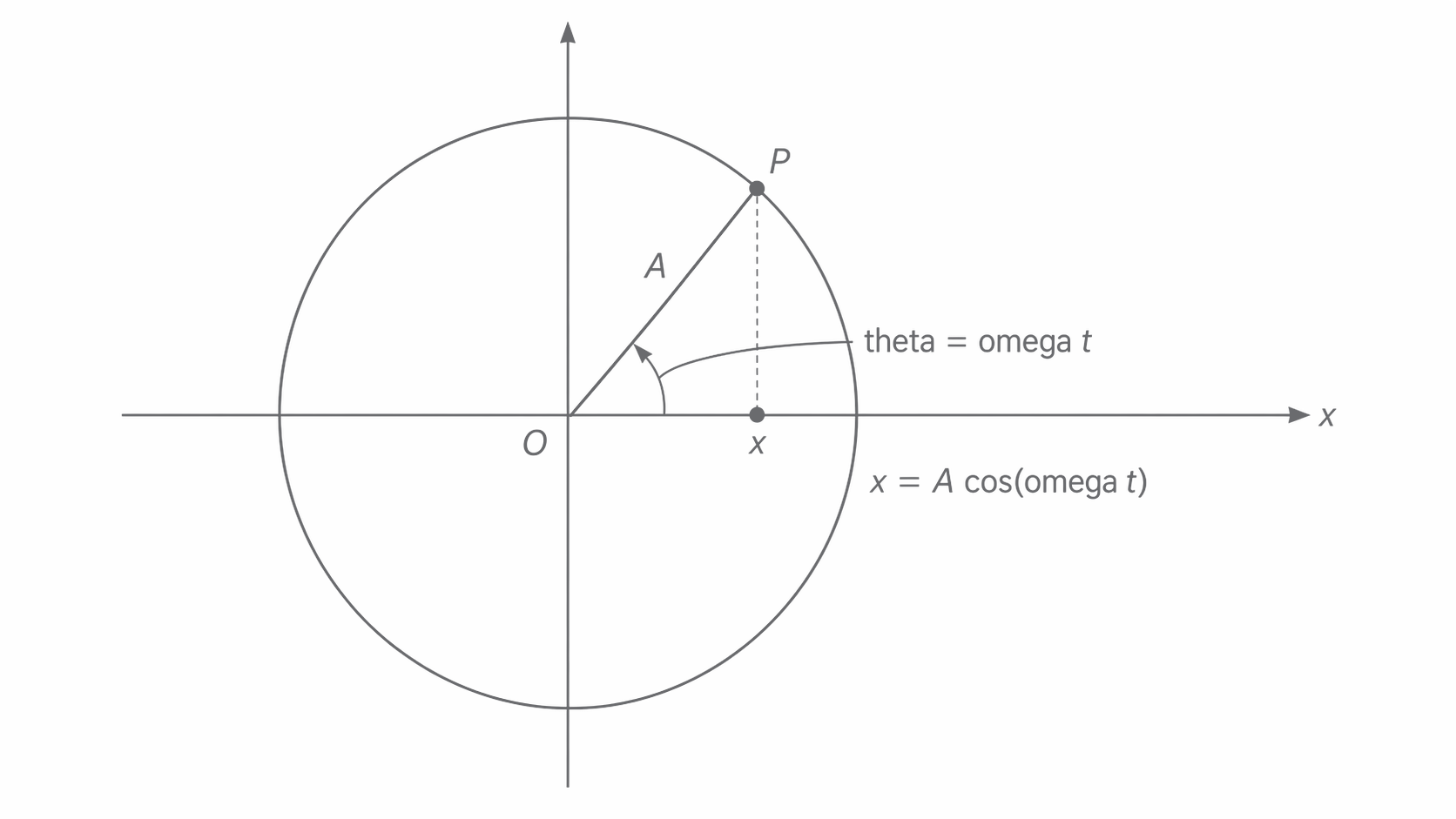
At time , if P has moved through angle from the positive -axis, then the -coordinate of P is:
The centripetal acceleration of P has magnitude and is directed towards the centre. Its component along the -axis is , which is exactly the defining equation of SHM.
This is why — originally the angular velocity of circular motion — appears as the angular frequency in SHM, and why the constant of proportionality in is specifically .
Piston engines convert between rotational and linear motion. A piston connected to a rotating crankshaft via a connecting rod undergoes approximately simple harmonic motion along the cylinder axis. The displacement of the piston from its mid-stroke position can be modelled as , where is the crank radius and is the angular velocity of the crankshaft. This model allows automotive engineers to predict the maximum piston speed () and the forces on engine components due to the maximum acceleration () at high RPM.
By this stage, the separate pieces should fit into one model: define SHM with the restoring acceleration, describe the motion with the displacement equation, and then use gradients or phase differences to move between the graphs.