RP04 - Determination of the Young Modulus
The Young modulus is the single number that tells you how stiff a material is --- how much it resists being stretched or compressed. In this required practical you will load a thin wire with known masses, measure tiny extensions to the nearest tenth of a millimetre, and extract the Young modulus from a straight-line graph. Every step, from choosing a long wire to reading a micrometer correctly, exists for a reason, and understanding those reasons helps you judge whether your result is trustworthy.
Part 1 --- The Physics Behind the Practical
When a tensile force is applied to a wire of original length and cross-sectional area , the wire extends by . Two ratios capture what is happening inside the material independently of the wire's dimensions.
Tensile Stress
The force per unit cross-sectional area acting on a material, measured in pascals (Pa).
For the same pulling force, a smaller cross-sectional area gives a larger stress.
Tensile Stress
Stress tells you how concentrated the pull is. A 10 N force on a thick cable produces much less stress than the same 10 N force on a very thin wire.
Tensile Strain
The fractional change in length of a material when a tensile force is applied. Strain has no units.
Strain tells you how much the material has deformed relative to its original size. A 1 mm extension on a 2 m wire is a much smaller strain than a 1 mm extension on a 10 cm wire.
The original length appears in the denominator, which is why strain has no units.
Tensile Strain
The Young modulus links the two.
Young Modulus
This equation is usually provided on the data sheet, but you must be able to rearrange and use it fluently. is a material property --- it does not depend on the wire's length or thickness, only on the substance it is made from. Steel has ; copper has .
Linearisation for graphical analysis
Rearranging the Young modulus equation to isolate the measured quantities:
This has the form where:
- (extension, plotted on the -axis)
- (applied force, plotted on the -axis)
- gradient
Therefore:
Young Modulus from Graph Gradient
Alternatively, if you plot on the -axis against on the -axis (which some mark schemes prefer), the gradient and so . Either convention is acceptable provided you are consistent.
Short exam link: stress--strain graphs and energy
This practical is usually analysed with an extension--force graph, but sometimes the same data are converted into stress and strain. In that case, the straight-line region still represents Hooke's law behaviour.
Energy per Unit Volume from Stress--Strain Graph
(valid in the linear region where Hooke's law holds)
This is because , and dividing both sides by the volume gives . The key exam check is to read the axis labels carefully: area under a force--extension graph gives energy in joules, whereas area under a stress--strain graph gives energy per unit volume in .
Part 2 --- Equipment, Setup, and Method
Equipment list
| Item | Purpose |
|---|---|
| Two lengths of steel wire (~1.5 m, ~0.45 mm diameter) | Test wire and comparison wire |
| Ceiling beam or strong overhead support | Suspension point for both wires |
| Wire clamps (4) | Secure each wire to the beam and to the scale/vernier |
| Millimetre scale with sliding vernier | Measure extension to |
| Micrometer screw gauge () | Measure wire diameter |
| Metre ruler () | Measure original length of test wire |
| Slotted masses (0.5 kg or 1 kg increments) | Apply known loads |
| Two mass hangers (1 kg each) | Pre-tension both wires |
| Safety goggles | Eye protection if wire snaps |
| Sand tray | Catches falling masses |
Apparatus diagram
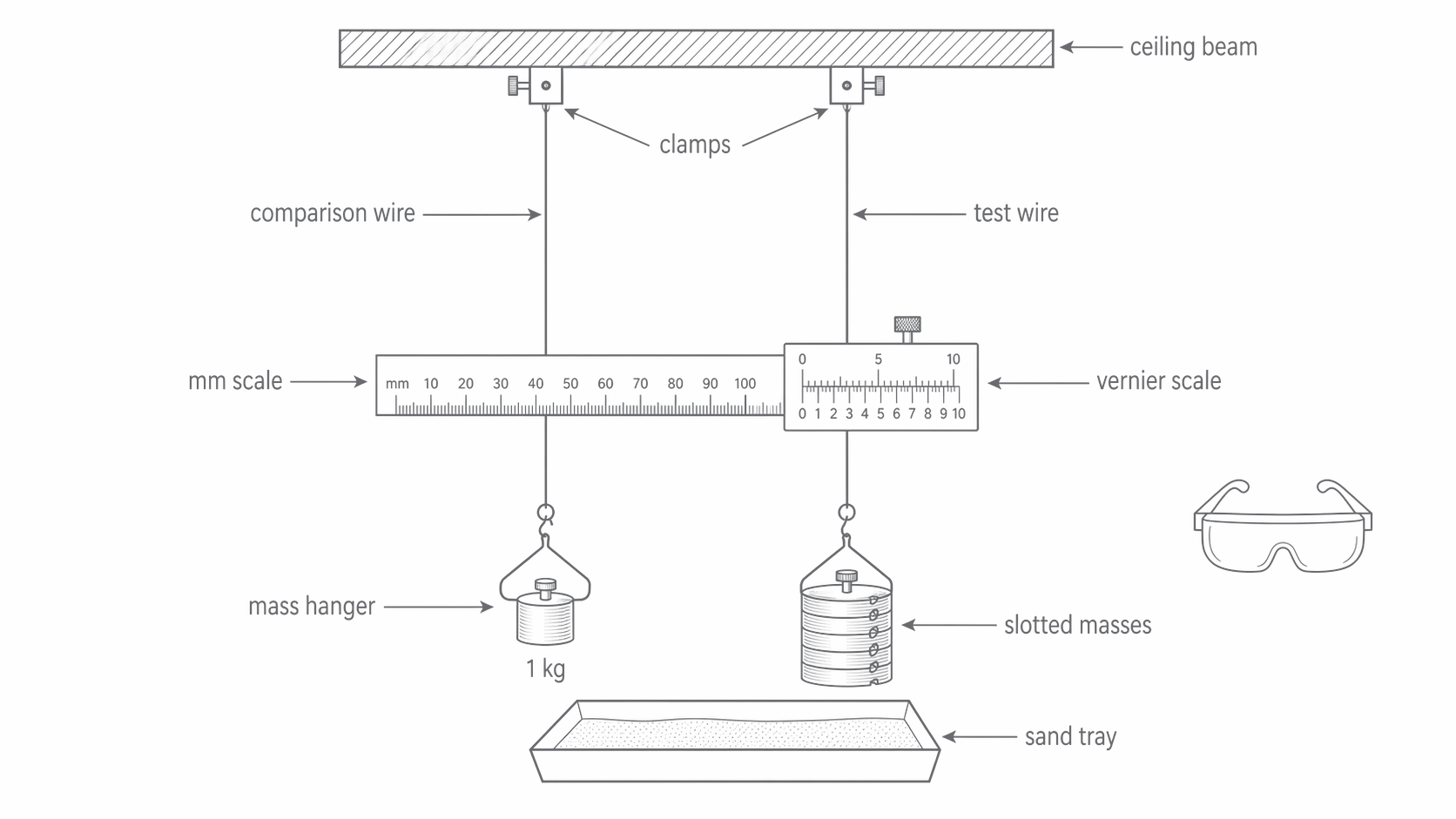
The figure below shows the standard two-wire setup; notice how the comparison wire and the scale-vernier pair let you measure the test wire's true extension while cancelling beam movement and thermal effects.
[DIAGRAM: asset_name: RP 04 - Determination of the Young Modulus by a Simple Method - Diagram 1; asset_slug: RP 04 - Determination of the Young Modulus by a Simple Method - Diagram 1; recommended_method: retained_png; description: Two long wires hang vertically side-by-side from a rigid ceiling beam. The left wire is labelled "comparison wire" and the right wire is labelled "test wire". Both are clamped to the beam at the top. A horizontal millimetre scale is clamped to the comparison wire at the bottom; a vernier slider is clamped to the test wire at the same height and slides against the scale. The comparison wire supports a single 1 kg hanger (to keep it taut). The test wire supports a hanger with a stack of slotted masses. A sand tray sits on the floor beneath the masses. Safety goggles are shown beside the setup. Labels: ceiling beam, clamps, comparison wire, test wire, mm scale, vernier scale, mass hanger, slotted masses, sand tray.]
Step-by-step method
-
Set up the two-wire system. Clamp both wires to the ceiling beam so they hang vertically, side by side, with the scale-and-vernier arrangement connecting them at the bottom.
- Why two wires? The comparison wire compensates for any sagging of the beam under load and for thermal expansion. Without it, a warm room could cause the beam to sag or the wire to lengthen, producing a false "extension". The comparison wire experiences the same environmental changes, so the vernier reading only reflects the true extension caused by the added mass.
-
Hang a 1 kg mass hanger from each wire. This pre-tensions both wires, removing any kinks and ensuring they hang straight.
- Why pre-tension? A kinked wire will "extend" as kinks straighten out, giving false readings that are not true elastic extension. Pre-tensioning ensures you are only measuring genuine elastic strain from the start.
-
Measure the original length of the test wire from the clamp at the beam down to the vernier clamp, using the metre ruler. Record in metres.
- Why measure to the vernier clamp? This is the length of wire that is actually stretching. Any wire above the beam clamp is not under the test load.
-
Record the initial vernier scale reading . This is your zero reference.
-
Add a 1 kg slotted mass to the test wire hanger. Wait a few seconds for the wire to stop oscillating, then read the new vernier position . The extension is .
- Why wait? The mass causes the wire to bounce briefly. Reading while oscillating introduces random error.
-
Continue adding masses in equal increments (e.g. 1 kg each time) up to about 7--8 kg total on the test wire, recording the vernier reading after each addition.
-
Unload the wire by removing masses one at a time, recording the vernier reading at each step.
- Why unload? Comparing loading and unloading readings checks whether the elastic limit has been exceeded. If unloading readings are larger than loading readings for the same mass, the wire has been permanently deformed and those data points must be discarded. If they match, the wire was within its elastic limit and you can average loading/unloading values to reduce random error.
-
Measure the wire diameter using the micrometer screw gauge at a minimum of six different positions along the wire (and at different orientations at each position in case the cross-section is not perfectly circular). Record all readings and calculate the mean diameter .
- Why multiple positions and orientations? The wire may not be perfectly uniform. Averaging reduces the effect of any localised variation.
- Why a micrometer? A ruler cannot resolve . Since the diameter is small (~0.45 mm), even a error represents a ~2% uncertainty in diameter, which doubles to ~4% in the area calculation.
-
Calculate the cross-sectional area .
-
Plot extension against the added load from the slotted masses and draw an unconstrained line of best fit. The theoretical relationship passes through the origin, but a measured best-fit line should not be forced through it; a significant intercept can reveal a zero offset or other systematic effect.
If your zero reading was taken with the hanger already attached, the hanger provides the baseline tension and the changing force on the graph is the force from the added slotted masses only.
Use the value of stated in the question or data sheet. If none is specified, is a sensible value to use for school practical calculations.
Why use a long, thin wire?
This is a common focus in practical discussions because a long, thin wire gives a larger extension for a given load, making the extension large enough to measure accurately.
Quantitatively, . For a fixed force and material:
- Doubling doubles --- a longer wire gives a larger, more measurable extension.
- Halving the diameter makes one quarter as large (since ), which quadruples .
If the wire were short and thick, extensions would be fractions of a millimetre --- far too small to measure reliably even with a vernier, leading to enormous percentage uncertainties.
Alternative methods
A common alternative is a horizontal bench method where the wire is clamped at one end, run across the bench over a pulley, and loaded with hanging masses. A travelling microscope or marker-and-ruler system measures the extension. This method is simpler to set up but less precise because friction at the pulley can reduce the effective tension, and the wire sags under its own weight. The vertical two-wire arrangement remains the standard method.
Part 3 --- Variables, Controls, and Experimental Design
| Variable type | Description |
|---|---|
| Independent variable | Applied force on the test wire, varied by adding slotted masses in increments of 1 kg (giving from approximately 10 N to 80 N) |
| Dependent variable | Extension of the test wire, measured using the vernier scale to |
| Controlled: Wire material | Use the same test wire throughout; do not swap wires between readings. Different materials have different Young moduli. |
| Controlled: Wire length | Measure once and do not alter the clamping points. If changes, the gradient changes even though has not. |
| Controlled: Wire diameter | Use a single uniform wire. If the wire had a varying cross-section, stress would not be uniform along its length. |
| Controlled: Temperature | The comparison wire compensates for thermal expansion, but avoid draughts or heat sources near the apparatus. Temperature changes could alter slightly and cause differential expansion. |
| Controlled: Loading method | Add masses gently and centrally to the hanger to avoid lateral oscillation, which could cause the wire to rub on the vernier and give false readings. |
Repeats: Load and unload the wire at least once (giving two sets of extension readings for each mass). If time allows, repeat the entire loading--unloading cycle a second time. Averaging loading and unloading values reduces random error in the extension readings and confirms the wire has not exceeded its elastic limit.
Suitable range: Use enough mass increments (at least 6--8 different loads) to produce a clear spread of data points on the graph. The maximum load should be chosen so that the wire does not exceed its elastic limit --- check by comparing loading and unloading values.
Part 4 --- Expected Results, Graphs, and Interpretation
Sample results table
The standard school setup for this required practical is the vertical two-wire apparatus described above. The sample numbers below come from a horizontal copper-wire version of the same experiment and are included purely to demonstrate the graph and calculation steps; once you have measured force and extension, the Young modulus analysis is the same.
Using sample data for a copper wire (, ):
| Mass / kg | Force / N | Extension / mm |
|---|---|---|
| 0.200 | 1.96 | 0.50 |
| 0.400 | 3.92 | 1.00 |
| 0.600 | 5.89 | 1.60 |
| 0.800 | 7.85 | 2.10 |
| 1.000 | 9.81 | 2.70 |
| 1.200 | 11.77 | 3.50 |
| 1.400 | 13.73 | 4.00 |
| 1.600 | 15.70 | 5.00 |
Graph
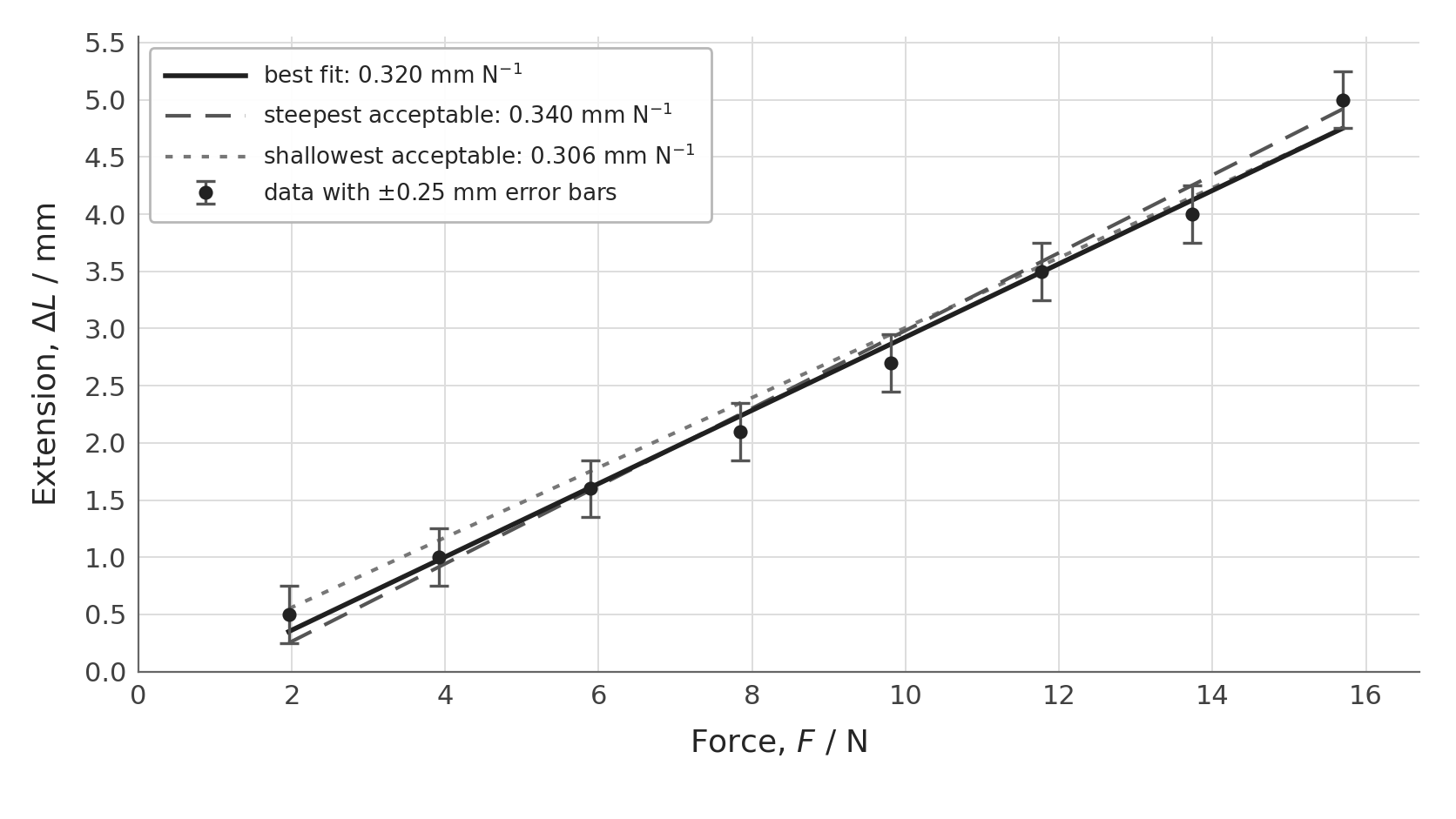
The graph below shows the expected straight-line trend. For this illustrative horizontal setup, the vertical error bars are , representing the estimated uncertainty from the resolution and repeat-to-repeat spread of the extension readings. The unconstrained best-fit line is shown with independently chosen steepest and shallowest acceptable lines that intersect every error bar.
[DIAGRAM: asset_name: RP 04 - Determination of the Young Modulus by a Simple Method - Diagram 2; asset_slug: RP 04 - Determination of the Young Modulus by a Simple Method - Diagram 2; recommended_method: deterministic_chart; description: Monochrome graph of extension / mm against force / N for eight sample measurements. Every point has a visible vertical uncertainty bar of mm. An unconstrained best-fit line has gradient 0.320 mm N and a negative intercept. Independently calculated dashed steepest and dotted shallowest acceptable lines intersect every error bar; neither is automatically constrained through the origin. Axes, units, line identities, and gradients are clearly labelled.]
Interpretation
The graph should be linear over the elastic range. The sample best-fit line is not forced through the origin and has a negative intercept, which could indicate a zero offset or another systematic effect. Its gradient still equals , from which the Young modulus is extracted.
If the line curves upward at high loads, the wire has exceeded its limit of proportionality. Data points in the curved region should be excluded from the gradient calculation.
The physical reason for the straight-line relationship is that, within the elastic limit, atomic bonds in the metal lattice behave like tiny springs. The macroscopic extension is the sum of billions of these tiny atomic-level stretches, and since each atom--atom "spring" obeys Hooke's law, so does the entire wire.
Civil and structural engineers determine the Young modulus of steel reinforcement bars and cable samples before using them in bridges and buildings. A test piece is loaded in a universal testing machine (essentially a sophisticated version of this experiment), and the stress--strain curve is recorded to confirm the steel meets the required stiffness specification.
Stress--strain graph interpretation
If you convert the same measurements to stress and strain, the gradient of the straight-line region is directly. For this practical, the important point is that only the linear region should be used to determine Young modulus.
The area under the linear portion of the stress--strain graph, a triangle of base and height , gives --- the elastic strain energy stored per unit volume.
Part 5 --- Worked Example with Full Calculation
Using the sample data: , .
Step 1: Calculate the cross-sectional area
Step 2: Determine the gradient
From the graph, select two widely separated points on the best-fit line (not data points, but points on the line itself).
Taking approximately and from the unconstrained best-fit line:
Step 3: Calculate the Young modulus
Step 4: Compare with the reference value
The reference Young modulus for copper is approximately .
This is well within typical experimental uncertainty, indicating that the method is sound and the wire was within its elastic limit throughout.
Step 5: Energy stored in the wire
Suppose the wire is loaded to with extension .
This energy is stored as elastic potential energy in the stretched atomic bonds. If the wire is unloaded within the elastic limit, all of this energy is recovered. On a force--extension graph this energy equals the triangular area under the line.
For the same copper wire, the stress at 9.81 N is , and the strain energy stored at an extension of 2.7 mm is . This is a good reminder that the same dataset can be used to extract stiffness, stress, and stored energy.
Part 6 --- Uncertainty and Error Analysis
Systematic errors
| Error | Direction of effect | How to identify |
|---|---|---|
| Zero error on the micrometer | Diameter reads consistently too high or too low, shifting and hence in one direction | Check the micrometer reads zero when closed (or record the zero error and subtract it from every reading) |
| Kinks in the wire | Extension appears larger than true elastic extension, making appear lower | Pre-tension both wires; inspect visually before starting |
| Friction at the vernier | Vernier may stick, giving readings that consistently lag behind the true extension | Tap the vernier gently before each reading; ensure the slider moves freely |
| Inaccurate value of | If at your location, all force values are shifted | Use the local measured value of if available; at A-level, use |
Random errors
| Error | Effect | How to reduce |
|---|---|---|
| Difficulty reading the vernier exactly | Extension values scatter above and below the true value | Take loading and unloading readings and average; repeat the experiment |
| Wire oscillating when mass is added | Reading taken before wire has settled | Wait for oscillations to die out before reading |
| Variation in wire diameter | Different readings at different points along the wire | Measure diameter at 6+ positions and orientations; use the mean |
| Parallax when reading the scale | Random in either direction | Read the vernier at eye level, perpendicular to the scale |
Full uncertainty calculation (worked through with numbers)
Uncertainty in diameter :
Suppose six micrometer readings (in mm) are: 0.273, 0.275, 0.274, 0.272, 0.276, 0.274.
Mean .
The range is , so the uncertainty from scatter is .
The micrometer's resolution is , giving an instrument uncertainty of (half the smallest division).
The scatter-based uncertainty () is smaller than the instrument uncertainty (), so we use the larger value: .
Uncertainty in area :
Since , and , the percentage uncertainty in is double the percentage uncertainty in :
The diameter is squared in the area formula, so its percentage uncertainty is doubled when you calculate the area. That makes diameter an important contributor, but you should still compare the actual percentage uncertainties in the data rather than assume it is always the largest term.
Uncertainty in length :
, measured with a metre ruler ().
This is negligible compared to the uncertainties in and .
Uncertainty in gradient (from the graph):
Draw the steepest and shallowest acceptable straight lines that intersect the uncertainty bars. Do not force either line through the origin.
For the plotted sample, the best-fit gradient is , the steepest acceptable gradient is , and the shallowest acceptable gradient is .
Using half the range as a symmetric estimate of the gradient uncertainty:
Combining uncertainties for :
Since , and , , and the gradient are all multiplied or divided:
So if :
The reference value of lies within this range, confirming the result is consistent with the known value.
As a quick check on the diameter calculation, readings of 0.44, 0.46, 0.45, 0.44, 0.45, and 0.46 mm give a mean diameter of . The half-range is , so the percentage uncertainty in is , and the percentage uncertainty in the cross-sectional area is therefore because the diameter is squared.
Sources of error and improvements table
| Source of error | Type | Effect on result | Improvement |
|---|---|---|---|
| Micrometer zero error | Systematic | All diameter readings shifted by a fixed amount, giving an incorrect area and hence incorrect | Check and record the zero error before use; subtract it from all readings |
| Wire not perfectly uniform in cross-section | Random | Different diameter values at different points; area calculation uses an imperfect average | Measure diameter at 6+ points and orientations; reject wire if range exceeds ~5% of mean |
| Difficulty reading small extensions on vernier | Random | Scatter in values, increasing scatter on graph | Use a travelling microscope instead of vernier for better resolution; take loading and unloading readings and average |
| Exceeding the elastic limit at high loads | Systematic | High-load data points deviate from linearity; gradient too steep (for vs graph), giving too low | Compare loading and unloading readings; exclude any points where unloading extension exceeds loading extension |
| Thermal expansion of the wire during the experiment | Systematic | Wire appears to extend more than expected, making appear lower | Use the comparison wire system; perform the experiment in a temperature-stable environment |
| Mixing up baseline tension and added load | Systematic if treated inconsistently | If the zero reading is taken with the hanger already attached, the graph should use the force from the added slotted masses only; mixing this with total load gives inconsistent force values | Decide on one convention before starting: either take extensions from zero load and use total load, or take a baseline with the hanger attached and use only the added force |
Part 7 --- Pulling the Practical Together
Most questions on this practical come back to the same chain of reasoning: measure the wire's geometry carefully, apply a range of known forces, measure the extensions as precisely as possible, and then use the graph gradient to separate the material property from the dimensions of the sample.
The common checks are whether you can justify the comparison wire, explain why the wire should be long and thin, recognise when the elastic limit has been exceeded, and decide which measured quantity is contributing most to the uncertainty in the final value of .
The Young modulus is determined by plotting extension against force for a loaded wire, extracting the gradient, and using . The comparison wire, long thin test wire, micrometer for diameter, and vernier for extension each serve a specific purpose --- understanding why earns marks; memorising what does not.
If you can explain why each piece of apparatus is there, you are much less likely to get stuck when the practical is described in an unfamiliar way.
Use that same idea when answering uncertainty questions: do the arithmetic first, then decide which source is largest from the numbers rather than from a rule of thumb.
A full method question then asks you to connect the measurements, the graph, and the error-reduction steps into one coherent answer.
The same practical logic is used well beyond the school lab whenever engineers need a reliable value for stiffness before choosing a material for a structure.
Materials scientists in the aerospace industry use tensile testing (the industrial-scale version of this practical) to determine the Young modulus and ultimate tensile strength of titanium alloys, carbon-fibre composites, and aluminium alloys. Each batch of material is tested to ensure it meets the stiffness and strength specifications before being used in aircraft structures where failure could be catastrophic.