RP01 - Stationary Waves on a String
Every stringed instrument you have ever heard works because of the physics in this practical. When you pluck a guitar string, progressive waves travel in both directions, reflect off the fixed ends, and superpose to form a stationary wave. The pitch of the note — its frequency — depends on three things: the length of the vibrating section, the tension in the string, and how heavy the string is per unit length. In this Required Practical you will vary one of these factors, measure the resonant frequency, and use graphical analysis to determine the wave speed on the string.
Part 1 — The Physics Behind the Practical
How stationary waves form on a string
When a vibration generator drives one end of a taut string, it sends a continuous progressive transverse wave along the string. This wave reflects at the far fixed end (the bridge or pulley), and the reflected wave travels back. The incident and reflected waves are identical in frequency, wavelength, and amplitude but travel in opposite directions. Where they meet, they superpose.
Stationary (Standing) Wave
A wave pattern formed by the superposition of two progressive waves of equal frequency, wavelength, and amplitude travelling in opposite directions. Energy is not transferred along the wave; instead, it is stored in sections that oscillate between nodes.
At certain points the two waves always cancel — these are nodes (points of permanent zero displacement). Midway between every pair of adjacent nodes are antinodes where the displacement is a maximum. Because both ends of the string are fixed, they must both be nodes. This boundary condition restricts which wavelengths — and therefore which frequencies — can sustain a stationary wave.
The first harmonic and the key equation
The simplest pattern that satisfies "node at each end" is a single loop: one antinode in the centre, one node at each end. The distance between adjacent nodes is half a wavelength, so for a string of vibrating length :
The wave speed on the string is related to frequency and wavelength by . Substituting :
First Harmonic Frequency
This is the central equation of the practical. It tells you that the resonant frequency of the first harmonic is inversely proportional to the vibrating length, and directly proportional to the wave speed.
What determines wave speed?
The speed of a transverse wave on a string depends only on two properties of the string: the tension pulling it taut, and the mass per unit length (how heavy the string is per metre). The relationship is:
Wave Speed on a String
Think about why this makes physical sense. Greater tension means the string snaps back more forcefully when displaced, so disturbances propagate faster — higher . A heavier string (larger ) has more inertia per metre, so it responds more sluggishly to the restoring force — lower .
Combining the two equations gives the master equation for this practical:
Complete First Harmonic Equation
This single equation contains all three independent variables the specification asks you to investigate: length , tension , and mass per unit length .
Linearisation — making the data give a straight line
Examiners love to test whether you can rearrange a curved relationship into a straight-line form . Here is how it works for each possible investigation.
Investigation 1 — varying length (constant and )
Starting from , rearrange to:
Plot (y-axis) against (x-axis). This gives a straight line through the origin with gradient .
Equivalently, the AQA handbook suggests plotting against :
This also gives a straight line through the origin, with gradient , so .
Both approaches are valid — AQA accepts either. The key insight is the same: because , , and are all constant, and have an inverse relationship, and plotting one against the reciprocal of the other produces a straight line.
Investigation 2 — varying tension (constant and )
From , squaring both sides:
Plot (y-axis) against (x-axis). Straight line through the origin, gradient .
Investigation 3 — varying mass per unit length (constant and )
Plot against . Straight line through the origin, gradient .
To investigate mass per unit length experimentally, keep the vibrating length and the tension fixed, then repeat the resonance measurement using strings with different materials or thicknesses. Measure the mass and total length of each sample first so you can calculate for that string. Under the same tension, a larger gives a lower wave speed and therefore a lower first-harmonic frequency.
These three rearrangements matter because the graph you choose depends on which variable you vary and which ones you keep constant.
Part 2 — Equipment, Setup, and Method
Equipment list
| Item | Purpose |
|---|---|
| Signal generator | Produces an alternating electrical signal at a controllable frequency |
| Vibration generator (transducer) | Converts the electrical signal into mechanical vibrations of the string |
| Retort stand with heavy base or clamp + 2 kg counterweight | Supports the vibration generator; counterweight prevents toppling |
| Pulley (bench-mounted) | Redirects the string vertically so masses can hang freely |
| Wooden bridge | Defines one end of the vibrating section; must be at the same height as the vibration generator hole |
| Slotted masses (100 g on a hanger) | Provide a known, constant tension |
| Metre ruler (mm graduations) | Measures the vibrating length between bridge and vibration generator |
| String, approximately 1.5 m | The medium on which stationary waves form |
| Electronic top-pan balance (±0.1 g) | Measures the total mass of the string to calculate |
Setting up the apparatus
In the setup diagram below, notice which horizontal section counts as the vibrating length , and how the hanging mass sets the string tension through the pulley.
[DIAGRAM: asset_name: RP 01 - Investigation into the Variation of the Frequency of Stationary Waves on a String - Diagram 1; asset_slug: RP 01 - Investigation into the Variation of the Frequency of Stationary Waves on a String - Diagram 1; recommended_method: retained_png; description: Side view of the apparatus. From left to right: a retort stand with clamp holds a vibration generator. A string is threaded through the hole in the vibration generator and tied to the stand. The string extends horizontally to the right, passing over a wooden bridge (a small triangular wedge resting on the bench), then continues to a pulley clamped at the edge of the bench. The string hangs vertically downward from the pulley with a mass hanger (100 g) attached. The vibrating section of the string is the horizontal portion between the vibration generator and the bridge — label this length as . The signal generator is connected to the vibration generator by two leads. A 2 kg counterweight sits on the base of the retort stand. Label all components.]
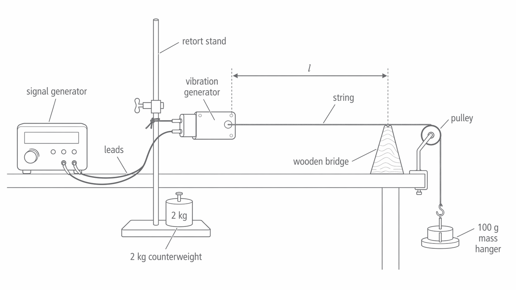
The string is tied to the stand, threaded through the hole in the vibration generator, then laid across the bench to the wooden bridge, over the pulley, and down to the hanging mass. The bridge should be at the same height as the vibration generator hole so the vibrating section is level, its length is easy to measure, and the stationary-wave pattern is clear. For a light string over a low-friction pulley, the tension is approximately uniform and set by the hanging load.
Step-by-step method
-
Warm up the signal generator by switching it on and leaving it for approximately 20 minutes. Why: the oscillator circuit inside drifts in frequency when cold. Allowing it to reach thermal equilibrium means the displayed frequency is stable and accurate.
-
Measure and record the total mass of the string using the top-pan balance before tying it to the apparatus. Also measure its full length (1.500 m). Why: you need the mass per unit length , and it is far easier to weigh the string before it is under tension.
-
Assemble the apparatus as described above. Hang a total load of 100 g from the pulley end. The tension is then approximately .
-
Set the vibrating length by positioning the wooden bridge exactly 1.000 m from the vibration generator. Measure from the point where the string leaves the vibration generator to the top of the bridge using the metre ruler. Why: the vibrating section must have a node at each end — the vibration generator provides a very-small-amplitude node at one end, and the bridge forces a node at the other.
-
Slowly increase the frequency on the signal generator from zero. Watch the string carefully. At a certain frequency the string will burst into large-amplitude vibration with a single antinode in the centre — this is the first harmonic. Why: you are sweeping through frequencies until you hit the resonant condition where .
-
Fine-tune the frequency to find the exact resonance. The resonance is sharpest when the antinode amplitude is at its maximum. Read and record the frequency from the signal generator display. A small paper rider balanced at the centre can help here: at the first harmonic it is thrown off most clearly when resonance is strongest.
-
Shorten the vibrating length by moving the bridge 0.100 m closer to the vibration generator, giving . Repeat the frequency sweep and record the new resonant frequency.
-
Continue reducing in steps of 0.100 m down to , recording each time. This gives six data points — a good range.
-
Repeat the entire set of measurements at least once more (ideally twice) and calculate the mean for each . Why: repeat readings reduce the effect of random errors and allow you to spot anomalies.
When you identify the first harmonic, describe the pattern precisely: a single loop with a node at each end and one antinode at the centre. That confirms you are using the mode for which applies.
Alternative methods
The AQA handbook notes two alternatives to the vibration generator setup:
- Wire and magnets: replace the vibration generator with a wire carrying alternating current between magnadur magnets. The wire experiences a periodic force due to the motor effect, driving the vibrations. The signal generator still controls the frequency.
- Fixed 50 Hz AC supply: if no signal generator is available, use a 50 Hz mains-frequency supply to drive the wire. Because the frequency is fixed, the investigation becomes: vary or to find the conditions that produce resonance at 50 Hz, and use the results to determine or the wire's density.
Safety
- The stand could topple if the hanging mass is too heavy relative to the stand's base. Use a 2 kg counterweight on the base or clamp the stand to the bench with a G-clamp.
- Keep fingers and loose clothing away from the vibrating string and pulley.
- Wear eye protection if using a wire rather than a string, as a wire under tension could snap.
Part 3 — Variables, Controls, and Experimental Design
The table below describes the standard version of this practical, where length is the independent variable.
| Variable type | Description |
|---|---|
| Independent variable | Vibrating length — varied from 1.000 m down to 0.500 m in 0.100 m steps (six values) |
| Dependent variable | Resonant first-harmonic frequency — read from the signal generator display (resolution typically ±0.1 Hz on a digital display, or ±0.5 Hz on an analogue dial) |
| Control 1: Tension | Keep the same hanging mass (100 g) throughout. Do not add or remove masses. Why: changing changes the wave speed , which would alter independently of . |
| Control 2: String type / | Use the same piece of string for every measurement. Do not swap to a different string. Why: a different string has a different mass per unit length , which changes . |
| Control 3: Harmonic mode | Always tune to the first harmonic (single loop). Higher harmonics resonate at higher frequencies for the same , which would introduce a systematic offset. Why: the equation only applies to the first harmonic. |
| Control 4: Signal generator warm-up | Ensure the signal generator has been on for 20 minutes or more before taking readings. Why: frequency drift during warm-up would create a systematic error in early readings. |
| Control 5: Bridge and generator height | Keep the bridge at the same height as the vibration generator hole. Why: this keeps the vibrating length well defined, makes the wave pattern easier to see, and reduces rubbing or twisting of the string. |
How to vary tension in a workable method
The standard student sheet varies length, but the same apparatus can also be used to investigate tension directly.
- Keep the same string throughout so stays constant.
- Keep the same vibrating length throughout, for example .
- Change only the hanging mass, for example in steps from 100 g to 350 g, and calculate the tension each time using .
- For each tension, sweep the frequency to the first harmonic and record the resonant frequency.
- Repeat each reading and calculate the mean value of .
- Plot against . A straight line through the origin supports the model .
The same logic can be turned round for mass per unit length.
How to vary mass per unit length in a workable method
- Keep the same vibrating length throughout, for example .
- Keep the same hanging mass throughout so the tension stays constant.
- Use several strings or wires of different thicknesses or materials.
- Measure the mass and total length of each sample before fitting it, then calculate for each one.
- For each string, adjust the frequency until the first harmonic is produced and record the resonant frequency.
- Repeat and average the frequencies, then plot against .
For this version, the string itself changes, so the key check is that the length, tension, and harmonic mode are all kept the same while only is changed.
Number of repeats
Take at least two full sets of readings and calculate the mean frequency for each length. Three sets is better. Repeats allow you to identify anomalies (a reading far from the others) and to calculate a spread (half-range), giving a measure of random uncertainty.
Ensuring a suitable range
Six values of spanning 0.500 m to 1.000 m gives a factor-of-two range. When you plot against , the values range from 1.0 to 2.0 m — this is wide enough that the gradient of the best-fit line can be determined reliably. If your graph points are clustered in a small region, the gradient becomes very sensitive to scatter, which increases uncertainty.
Part 4 — Expected Results, Graphs, and Interpretation
Sample results table
The data below are taken from the AQA practical handbook for a 100 g hanging mass () with a string of mass 0.91 g and total length 1.500 m ().
| / m | / Hz | / m s | / m | / s |
|---|---|---|---|---|
| 1.00 | 20.5 | 41.0 | 1.00 | 0.0488 |
| 0.90 | 23.5 | 42.3 | 1.11 | 0.0426 |
| 0.80 | 26.5 | 42.4 | 1.25 | 0.0377 |
| 0.70 | 30.0 | 42.0 | 1.43 | 0.0333 |
| 0.60 | 34.5 | 41.4 | 1.67 | 0.0290 |
| 0.50 | 42.0 | 42.0 | 2.00 | 0.0238 |
Notice that the calculated wave speed is roughly constant at about 41–42 m s across all lengths. This is exactly what we expect: the wave speed depends on and , both of which are held constant. The small variation (41.0 to 42.4) is due to experimental uncertainty in reading .
What graph to plot
Option A (recommended by AQA handbook): (y-axis) against (x-axis)
From , taking reciprocals: .
This is in the form where:
- gradient
- y-intercept (the line should pass through the origin)
So .
Option B: (y-axis) against (x-axis)
From :
- gradient
- y-intercept
So .
Both are equally valid. The AQA student sheet suggests Option A, so we will use that in the worked example.
Expected graph shape
In the graph below, notice that the best-fit line should pass through the origin and that the gradient triangle is taken from the line itself, while the dashed worst acceptable line shows how gradient uncertainty is estimated.
[DIAGRAM: asset_name: RP 01 - Investigation into the Variation of the Frequency of Stationary Waves on a String - Diagram 2; asset_slug: RP 01 - Investigation into the Variation of the Frequency of Stationary Waves on a String - Diagram 2; recommended_method: retained_png; description: Graph with / m on the x-axis (ranging from 0 to 1.2) and / s on the y-axis (ranging from 0 to 0.06). Six data points are plotted showing a clear linear trend passing through or very close to the origin. A best-fit straight line is drawn through the points and the origin. The line has a positive gradient. The gradient triangle is drawn on the graph: a large right-angled triangle using two well-separated points on the best-fit line (not data points), with the rise labelled and the run labelled . Label the gradient as . A dashed "worst acceptable line" is also shown, drawn as the steepest line that still passes through all the error bars, to illustrate how gradient uncertainty is found.]
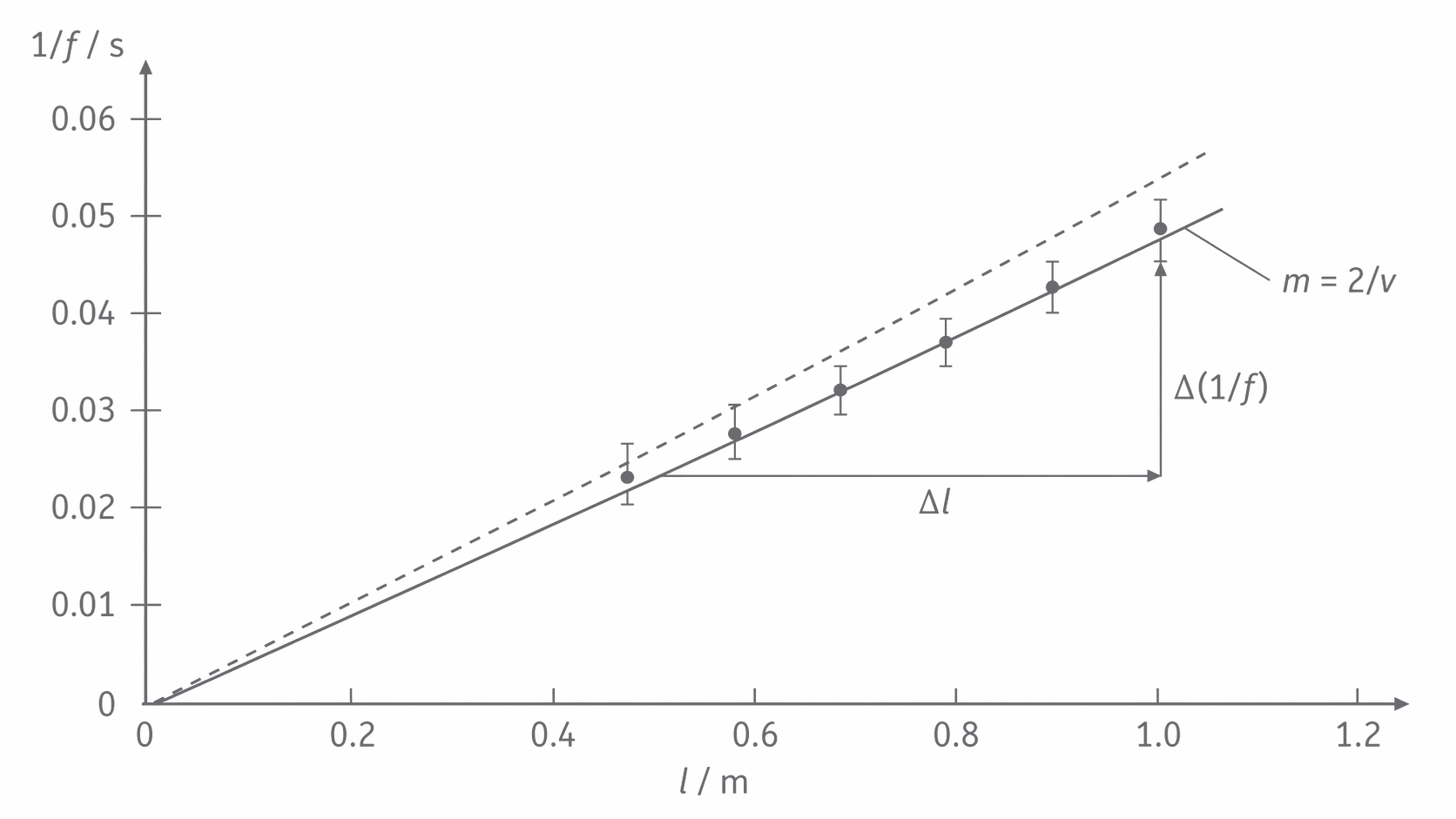
The graph should be a straight line through the origin. If the line has a noticeable y-intercept, this suggests a systematic error — most likely a zero error in the length measurement (for example, measuring from the wrong reference point on the vibration generator).
Physical explanation of the trend
As the vibrating length decreases, fewer half-wavelengths fit into the string at the first harmonic. Since , a shorter string means a shorter wavelength. The wave speed is unchanged (same tension, same string), so from , a shorter wavelength requires a higher frequency. This is why shorter guitar strings produce higher-pitched notes.
Guitar and violin design relies directly on this physics. Pressing a finger on a guitar fret shortens the vibrating length of the string, raising the first-harmonic frequency and therefore the pitch. Different strings on the same instrument have different mass per unit length (thicker strings for bass notes, thinner for treble), and tuning pegs adjust the tension . All three variables from this practical — , , — are used by musicians every day.
Part 5 — Worked Example: Full Calculation
We will work through the complete analysis using the AQA sample data.
Step 1: Calculate processed quantities
For each data point, calculate :
| / m | / Hz | / s |
|---|---|---|
| 1.00 | 20.5 | 0.04878 |
| 0.90 | 23.5 | 0.04255 |
| 0.80 | 26.5 | 0.03774 |
| 0.70 | 30.0 | 0.03333 |
| 0.60 | 34.5 | 0.02899 |
| 0.50 | 42.0 | 0.02381 |
Step 2: Plot the graph and determine the gradient
Plot (y-axis) against (x-axis). The points lie close to a straight line through the origin. Draw the best-fit line.
To calculate the gradient, pick two points far apart on the best-fit line (not necessarily data points). Using the first and last data points as an approximation:
Step 3: Calculate the wave speed from the gradient
From , we have gradient :
Step 4: Compare with the theoretical value
Using :
- Tension:
- String mass:
- String length:
- Mass per unit length:
Step 5: Calculate the percentage difference
The two values differ by only 0.5%, so they are in close agreement for this data set. Whether they agree within experimental uncertainty can be decided only after estimating the uncertainty in both determinations; percentage difference alone does not establish reliability or rule out systematic error.
The wave speed determined from the graph () is 0.5% below the theoretical prediction from (). This close agreement supports the model for these data; a conclusion about agreement within uncertainty requires an uncertainty estimate.
A single row of data is also a useful check before you rely on the whole graph.
Part 6 — Uncertainty and Error Analysis
This section matters because your conclusion is only convincing if you can show how large the uncertainties are and where the main errors come from.
Systematic errors in this practical
Systematic Error
An error that shifts all readings in the same direction by a consistent amount. It cannot be reduced by repeating measurements. It is identified by comparison with an accepted value or by checking for a non-zero y-intercept on a graph that should pass through the origin.
Specific systematic errors here:
- Zero error in length measurement: if you consistently measure from the wrong point (e.g., from the casing of the vibration generator rather than the point where the string exits), every length is offset by the same amount. This shifts the entire graph sideways and produces a non-zero y-intercept.
- Signal generator frequency calibration: if the signal generator reads systematically high or low (e.g., displays 20.0 Hz when the true frequency is 20.5 Hz), every frequency reading is offset. An oscilloscope can be used to independently check the signal generator's output frequency.
- Pulley friction or rubbing at the bridge: if the string does not move freely over the pulley or bridge, the tension in the vibrating section can be slightly less than the hanging weight. This makes the calculated wave speed come out too high if you still assume .
Random errors in this practical
Random Error
An error that causes readings to scatter unpredictably above and below the true value. It can be reduced by taking repeat measurements and averaging, or by improving the measurement technique.
Specific random errors here:
- Judging the resonant frequency: identifying the exact frequency at which the string vibrates with maximum amplitude is subjective. You might overshoot or undershoot slightly each time. This is the dominant source of random error in this practical.
- Reading the length: parallax when reading the metre ruler, or slight variation in where you judge the string to leave the vibration generator.
- Environmental vibrations: draughts, bench vibrations from nearby equipment, or bumping the apparatus can disturb the wave pattern.
Worked uncertainty calculation
Let us quantify the uncertainties using the sample data.
Uncertainty in length
The metre ruler has 1 mm graduations. The absolute uncertainty in a single length measurement is ±0.5 mm at each end (reading uncertainty), giving a total of ±1 mm for the distance between two points.
Percentage uncertainty at :
Percentage uncertainty at :
Notice that the percentage uncertainty doubles as the length halves — this is why shorter lengths give less precise results proportionally.
Uncertainty in frequency
The main source of uncertainty in is not the resolution of the signal generator (which might be ±0.1 Hz), but rather the difficulty of judging exactly when resonance occurs. A reasonable estimate is that the resonant frequency can be identified to within ±0.5 Hz. For example, at , :
At , :
Frequency uncertainty dominates over length uncertainty — this tells us that improving our ability to judge resonance (e.g., using a paper rider or stroboscope) would do more to improve accuracy than using a more precise ruler.
Uncertainty in wave speed
Since , and the factor of 2 is exact, the percentage uncertainty in is found by adding the percentage uncertainties in and :
At :
So for this single data point.
Uncertainty in
- , for a digital balance reading to 0.1 g. Percentage uncertainty: .
- , . Percentage uncertainty: .
The uncertainty in is dominated by the mass measurement, because the string is very light (less than 1 g) and the balance resolution is ±0.1 g.
Uncertainty in the theoretical speed
The uncertainty in is negligible compared with the uncertainty in , so:
So .
Uncertainty in the gradient
To find the uncertainty in the gradient from the graph, draw the worst acceptable line — the steepest (or shallowest) straight line that still passes through all the error bars on the data points. Then:
This propagates directly into the uncertainty in from the graph.
Sources of error and improvements
| Source of error | Type | Effect on results | Improvement |
|---|---|---|---|
| Difficulty judging exact resonant frequency by eye | Random | Scatter in values; dominant random error | Use a small paper rider on the string at the antinode — it is thrown off at resonance, giving a sharper indication. Alternatively, use a microphone and oscilloscope to detect maximum amplitude electronically. |
| Signal generator frequency drift (before warm-up) | Systematic | All readings shifted in one direction | Allow the signal generator to warm up for at least 20 minutes before taking any readings. |
| Zero error in length measurement | Systematic | Constant offset in ; non-zero y-intercept on graph | Use a set square to ensure the ruler is perpendicular to the string at the measurement points. Mark the exact points where the string contacts the bridge and exits the vibration generator. |
| String rubs strongly on the bridge or pulley | Systematic | Actual tension in the vibrating section is slightly less than the hanging weight, so calculations based on are inaccurate | Keep the bridge level with the generator, use a low-friction pulley, and check that the string moves freely |
| String mass measurement with low-resolution balance | Random (reading uncertainty) | Large percentage uncertainty in because string mass is very small | Use a balance with higher precision (±0.01 g). Alternatively, measure a longer piece of string and cut it after weighing. |
| Damping and overtones — string may vibrate in a higher harmonic without the observer noticing | Systematic | Measured would be a multiple of the true first-harmonic frequency, giving a that is too high | Always start from a very low frequency and increase slowly. Confirm the pattern is a single loop with one antinode. Compare with the predicted before recording. |
When suggesting an improvement, be specific about the equipment or technique and say how it reduces the uncertainty. For example, a more precise balance directly lowers the percentage uncertainty in because the string mass is so small.
Part 7 - Bringing It Together
A good set of results should show three linked ideas clearly: shorter strings need higher first-harmonic frequencies, greater tension raises the frequency, and a larger mass per unit length lowers it. When those trends match both the graph relationships and , the practical has tied the stationary-wave pattern to the wave-speed model successfully.
Engineers can estimate the tension in a stretched cable by measuring its resonant frequency. If the cable length and mass per unit length are known, the tension can be found from the same relationships used in this practical, without cutting or damaging the cable.
Musicians use the same physics every time they tune an instrument: they shorten the vibrating length, tighten the string, or swap to a string with a different mass per unit length.