9G - Estimating small changes

How can a derivative estimate a nearby square root or the effect of a tiny change in radius? You will use a tangent to estimate changes and new values, then compare estimates with exact calculations so that their accuracy is stated meaningfully.

A tangent as a local approximation

A tangent has the same gradient as a smooth curve at its point of contact, making it a useful approximation very close to that point.

Suppose $y=f(x)$ , and $x$ changes from $a$ to $a+h$ . The exact change is $f(a+h)-f(a)$ . On the tangent at $x=a$ , a horizontal change $h$ produces a vertical change equal to gradient times $h$ .

Small changes

For a sufficiently small change $\Delta x$ near a differentiable point $x=a$ ,

\Delta y\approx f'(a)\Delta x, \qquad f(a+\Delta x)\approx f(a)+f'(a)\Delta x.

The specification also writes this as $\mathrm{d}y\approx\frac{\mathrm{d}y}{\mathrm{d}x}\mathrm{d}x$ for small $\mathrm{d}x$ . Evaluate the derivative at the starting value. The symbol $\approx$ matters: a curved graph generally leaves an error.

[DIAGRAM: asset_name: A tangent estimates a nearby change; asset_slug: tangent-change; caption: Near x equals 3, the tangent to y equals x squared follows the curve closely; description: The curve y equals x squared and its tangent y equals 9 plus 6 times (x minus 3) are plotted close to (3,9). At x equals 3.2 a vertical gap separates tangent value 10.2 and curve value 10.24. A horizontal arrow marks delta x equals 0.2 and a vertical arrow marks tangent change 1.2. The gap 0.04 is labelled as the omitted square of delta x.]
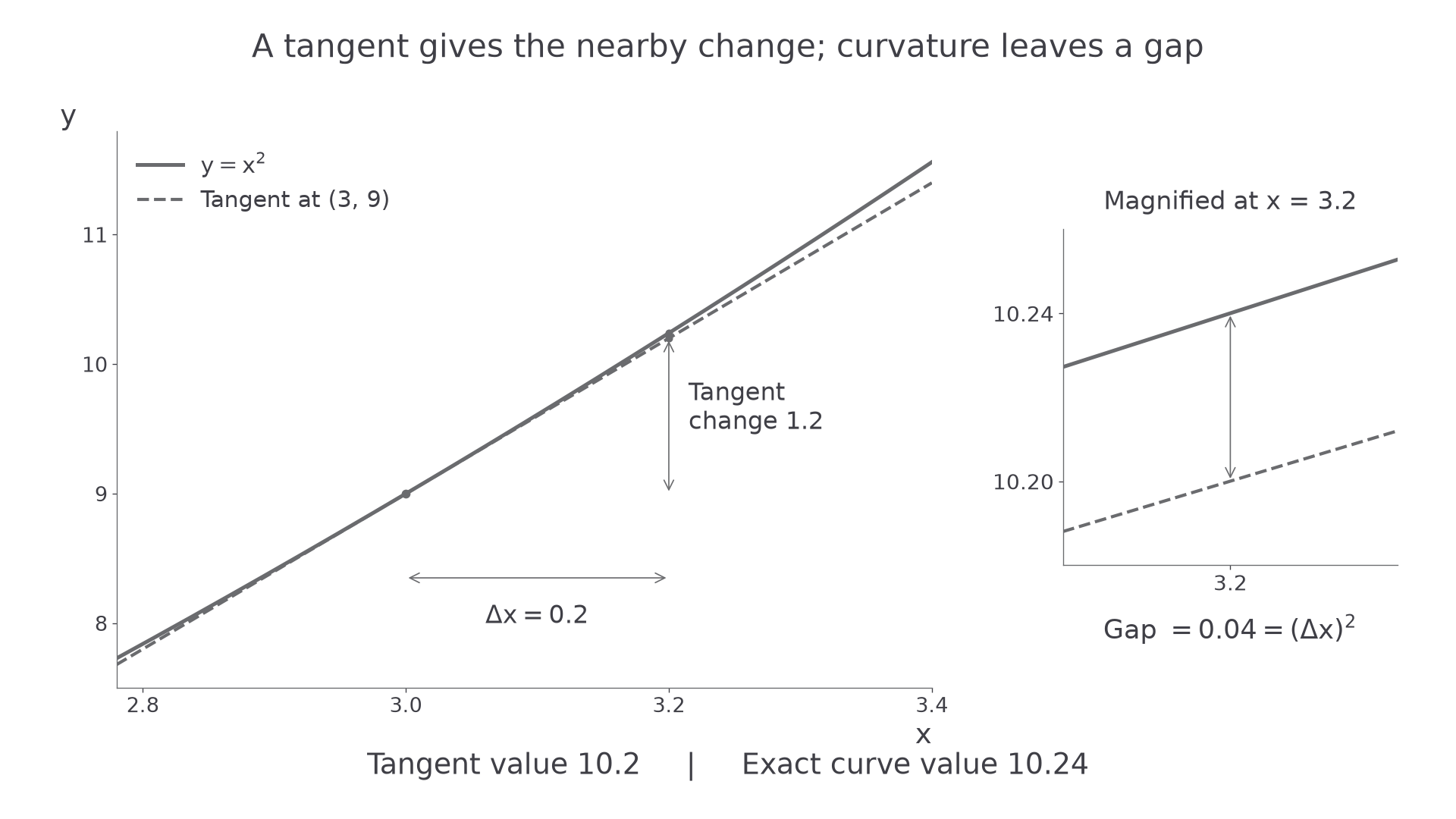
Near x equals 3, the tangent to y equals x squared follows the curve closely

Keep the sign of $\Delta x$ . If the input decreases, $\Delta x<0$ ; whether the output increases or decreases then depends on the gradient as well.

Worked example 1: a small increase

Question. For $y=x^2$ , estimate the change in $y$ when $x$ increases from $3$ to $3.02$ .

Plan. Use the gradient at the starting point, $x=3$ , and the small input change $0.02$ .

f'(x)=2x,\qquad f'(3)=6,\qquad \Delta x=3.02-3=0.02.

Hence

\Delta y\approx6(0.02)=0.12.

Answer. The estimated increase in $y$ is $0.12$ .

Check. The exact difference can be factored: $3.02^2-3^2=(3.02-3)(3.02+3)=0.02(6.02)=0.1204$ . The estimate is close because the secant gradient $6.02$ is close to the starting tangent gradient $6$ .

Now reverse the input change while keeping its size and the starting point. The derivative is unchanged, but the estimated change must reverse sign.

Worked example 2: a small decrease

Question. For $y=x^2$ , estimate the change in $y$ when $x$ decreases from $3$ to $2.98$ .

Plan. Use the same starting gradient $6$ , now with $\Delta x=-0.02$ .

\Delta y\approx f'(3)\Delta x=6(-0.02)=-0.12.

Answer. The estimated change is $-0.12$ , a decrease of $0.12$ .

Check. Exactly, $2.98^2-3^2=(2.98-3)(2.98+3)=-0.02(5.98)=-0.1196$ . Its sign agrees with the estimate. The secant gradient $5.98$ is again close to $6$ .

A change is a signed difference, not the new value of the function.

Estimating a change or a new value

An estimated change must be added to the starting quantity if the question asks for its new value.

Choose a nearby starting value where the function and derivative are easy to evaluate. For a square root, a nearby square number is useful. For percentage changes, first turn the percentage input change into an actual change, or divide the small-change equation by the starting output.

Worked example 3: a nearby square root

Question. Use differentiation at $x=25$ to estimate $\sqrt{25.2}$ .

Plan. Take $f(x)=\sqrt{x}$ , estimate its change from $25$ to $25.2$ , then add that change to $5$ .

f'(x)=\frac1{2\sqrt{x}},\qquad f'(25)=\frac1{10},\qquad \Delta x=0.2.

Therefore

\Delta y\approx\frac1{10}(0.2)=0.02, \qquad \sqrt{25.2}\approx5+0.02=5.02.

Answer. $\sqrt{25.2}\approx5.02$ .

Check. $5.02^2=25.2004$ , very close to the required $25.2$ . The exact root is therefore slightly below $5.02$ . The estimate is a new root value, whereas $0.02$ is only its estimated increase.

For a percentage increase in a geometric dimension, the output percentage need not be the same. A volume depends on three powers of a length.

Worked example 4: a percentage radius change

Question. A sphere initially has radius $10\,\mathrm{cm}$ . Its radius increases by $0.5\%$ . Use differentiation to estimate the increase in volume and the percentage increase in volume. Use $V=\frac43\pi r^3$ .

Plan. Convert the radius percentage to $\Delta r$ , multiply by $\frac{\mathrm{d}V}{\mathrm{d}r}$ at $r=10$ , and compare with the original volume.

\Delta r=\frac{0.5}{100}(10)=0.05\,\mathrm{cm}, \qquad \frac{\mathrm{d}V}{\mathrm{d}r}=4\pi r^2.

Thus

\Delta V\approx4\pi(10)^2(0.05)=20\pi\,\mathrm{cm^3}.

The starting volume is $V_0=\frac{4000\pi}{3}\,\mathrm{cm^3}$ , so

\frac{\Delta V}{V_0}\times100\% \approx\frac{20\pi}{4000\pi/3}\times100\%=1.5\%.

Answer. Increase approximately $20\pi\,\mathrm{cm^3}$ , or $1.5\%$ of the original volume.

Check. The exact fractional increase is $(1.005)^3-1=0.015075125$ , or $1.5075125\%$ . This is close to $1.5\%$ . Algebraically, dividing $\Delta V\approx4\pi r^2\Delta r$ by $V=\frac43\pi r^3$ gives $\frac{\Delta V}{V}\approx3\frac{\Delta r}{r}$ , explaining the factor of three.

Last Accessed

Number

Algebra

Series

Geometry

Trigonometry

Calculus

9G - Estimating small changes

A tangent as a local approximation

Estimating a change or a new value

Continue this lesson.

Learn faster with Nova