4B - Solving equations with graphs

What can you do when an equation has no convenient exact solution? Graphs turn equality into a visible meeting point. You will choose graphs that represent an equation, use a suitable straight line with logarithmic or exponential curves, and report solutions at an accuracy the graph supports.

Roots as intersections

How could you solve $x^3-3x=1$ when simple integer substitutions do not produce a root?

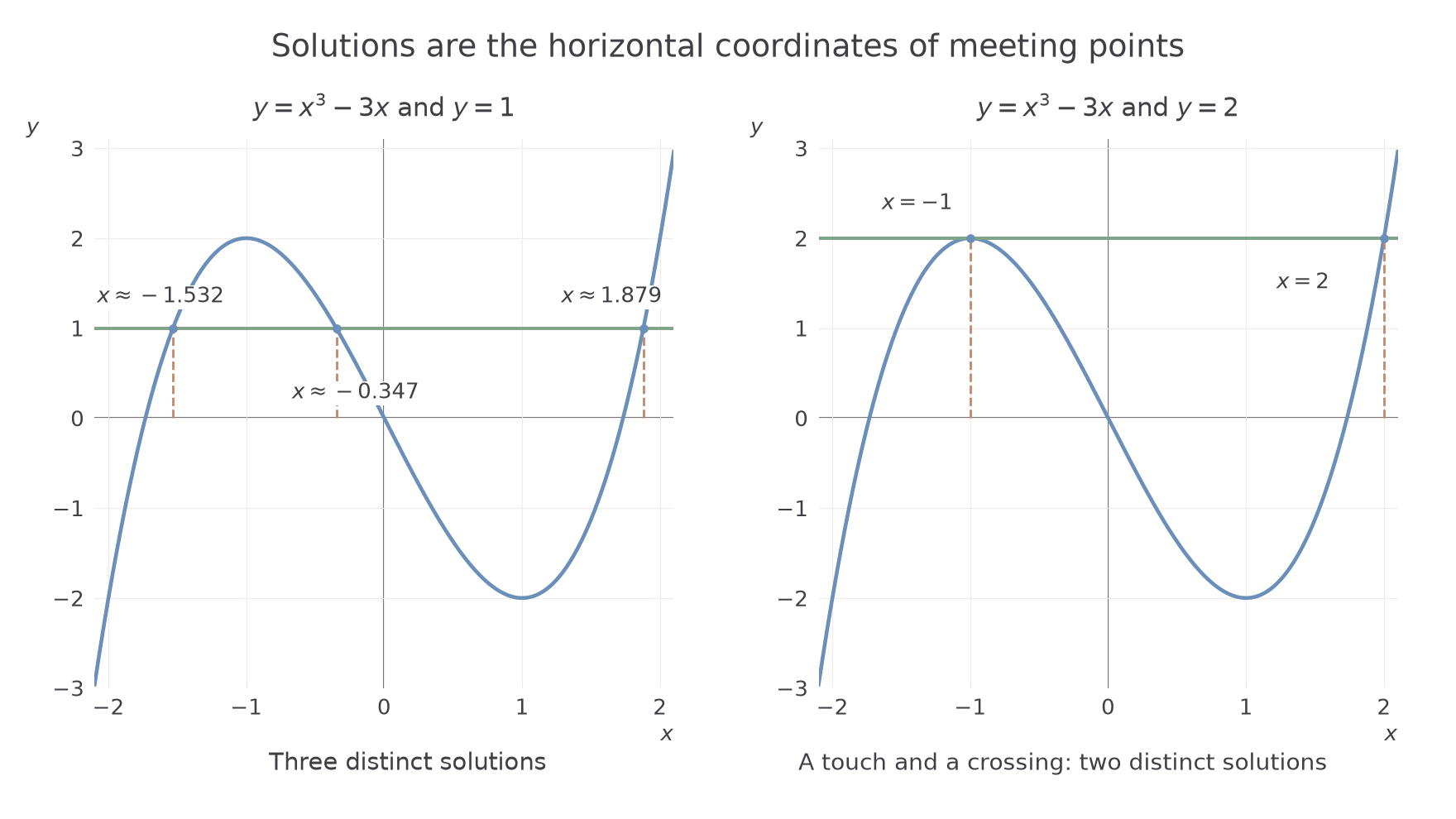
Plot $y=x^3-3x$ , then draw $y=1$ . Wherever the curves meet, their heights are equal, so the same input satisfies the original equation. There are three meeting points: the graph reveals solutions that one guessed value could miss.

Graphical solution

A solution of $f(x)=g(x)$ is the $x$ -coordinate of an intersection of $y=f(x)$ and $y=g(x)$ , provided both functions are defined there. A root of $f(x)=0$ is the special case where the second graph is the $x$ -axis.

Rearrange the equation to use the graph you have. If $y=x^3-3x$ is already drawn, solving $x^3-3x-1=0$ needs the line $y=1$ , rather than a new cubic. Choose a scale that shows all intersections in the requested interval and read their horizontal coordinates.

Worked example 1: three solutions from one curve

Question. Use $y=x^3-3x$ to solve $x^3-3x-1=0$ , for $-2.1\le x\le2.1$ , to $1$ decimal place.

Plan. Rearrange to make the plotted expression equal to a constant, then read all its intersections with that horizontal line.

x^3-3x-1=0\implies x^3-3x=1.

Draw $y=1$ . The left-hand graph below shows intersections at approximately $-1.53$ , $-0.35$ and $1.88$ . Round the horizontal readings as requested.

Answer. $x\approx-1.5$ , $-0.3$ and $1.9$ , to $1$ decimal place. Use the unrounded graph positions when rounding: the middle intersection is slightly greater than $-0.35$ .

Check. Substitution in $x^3-3x$ gives $1.008$ at $-1.53$ , $1.007$ at $-0.35$ and $1.005$ at $1.88$ . These nearby readings give heights close to the required $1$ ; the rounded answers are coarser.

Change just the constant from $1$ to $2$ . One horizontal line can meet a curve at a touch as well as at a crossing.

Worked example 2: a touching intersection

Question. Use the same cubic to solve $x^3-3x-2=0$ , for $-2.1\le x\le2.1$ .

Plan. Draw $y=2$ and count each distinct meeting point once.

x^3-3x-2=0\implies x^3-3x=2.

The right-hand graph shows a touch at $(-1,2)$ and a crossing at $(2,2)$ . Read the $x$ -coordinates, not the common height $2$ .

Answer. The graphical readings are $x\approx-1$ and $x\approx2$ . Substitution confirms the exact solutions $x=-1$ and $x=2$ .

Check. $(-1)^3-3(-1)=2$ and $2^3-3(2)=2$ . Also, $x^3-3x-2=(x+1)^2(x-2)$ , confirming a repeated root at $-1$ , counted once in the list of distinct solutions.

[DIAGRAM: asset_name: Horizontal lines turn a cubic into equation solutions; asset_slug: cubic-intersections; caption: Read all meeting points, including a touch, to solve the cubic equations; description: Two plots of y equals x cubed minus 3x on minus 2.1 to 2.1 show the horizontal lines y equals 1 and y equals 2. The first has three intersections with x-coordinates approximately minus 1.532, minus 0.347 and 1.879. The second touches at x equals minus 1 and crosses at x equals 2. Horizontal guide lines and vertical reading guides distinguish the height from the required x-coordinate.]
Read all meeting points, including a touch, to solve the cubic equations

Watch out

An intersection need not be a crossing. A line that touches the curve still gives a solution. For $f(x)=g(x)$ , report the input $x$ ; give both coordinates only if the question asks for the intersection point.

The opening equation has three real solutions in the displayed interval, even though none is an integer.

Equations involving logarithms or exponentials

A logarithmic or exponential equation can often be matched to a curve you have already drawn by finding the right straight line.

Consider the curve $y=\log_2(5-x)+1$ . Its logarithm needs $5-x>0$ , so $x<5$ . Use a calculator to build a table on $0\le x\le4.5$ , keeping extra digits until rounding the displayed values.

$x$	$0$	$0.5$	$1$	$1.5$	$2$	$2.5$	$3$	$3.5$	$4$	$4.5$
$\log_2(5-x)+1$	$3.32$	$3.17$	$3.00$	$2.81$	$2.58$	$2.32$	$2.00$	$1.58$	$1.00$	$0.00$

Plot the points on labelled axes and join them with a smooth curve. The table supplies points, not a series of straight segments. Nearer to $5$ the curve becomes steeper, so more closely spaced inputs help if that region is needed.

Transcendental equation

A transcendental equation involves a function such as a logarithm or exponential and is not simply a polynomial equation. Graphs can estimate solutions even when the usual algebraic methods do not isolate the unknown.

Logarithm laws are useful before drawing a line. On the stated domain, $5-x>0$ , so taking logs and using the power law preserves the following equations.

Worked example 3: finding the suitable line

Question. Use $y=\log_2(5-x)+1$ to solve $2^{x-2}=(5-x)^2$ on $0\le x\le4.5$ , to $1$ decimal place.

Plan. Take logarithms to base $2$ , then rearrange until one side is exactly the plotted expression.

\begin{aligned} 2^{x-2}&=(5-x)^2\\ x-2&=2\log_2(5-x) &&\text{take logs and use the power law}\\ \frac{x-2}{2}+1&=\log_2(5-x)+1 &&\text{divide by }2\text{, then add }1\\ \frac{x}{2}&=\log_2(5-x)+1 &&\text{simplify the line} \end{aligned}

Draw $y=x/2$ , for example through $(0,0)$ and $(4,2)$ . Its intersection with the decreasing curve is near $x=3.38$ .

Answer. $x\approx3.4$ , to $1$ decimal place.

Check. At the closer graphical reading $x=3.38$ , the two sides of the original equation are about $2.60$ and $2.62$ , agreeing within the reading accuracy. The intersection lies in the required interval and has $5-x>0$ .

Now change only the coefficient of $x$ in the exponent from $1$ to $2$ . The curve and table stay useful; the required line changes slope.

Worked example 4: changing the exponent

Question. Use the same curve to solve $2^{2x-2}=(5-x)^2$ on $0\le x\le4.5$ , to $1$ decimal place.

Plan. Repeat the logarithmic rearrangement and identify the new straight line.

\begin{aligned} 2x-2&=2\log_2(5-x) &&\text{take logs to base }2\\ x-1&=\log_2(5-x) &&\text{divide by }2\\ x&=\log_2(5-x)+1 &&\text{match the plotted expression} \end{aligned}

Draw $y=x$ , through $(0,0)$ and $(3,3)$ . This steeper line meets the curve near $x=2.39$ .

Answer. $x\approx2.4$ , to $1$ decimal place.

Check. At $x=2.39$ , $2^{2x-2}\approx6.87$ and $(5-x)^2\approx6.81$ . A small horizontal reading error changes the values, but their closeness supports the graphical estimate. The steeper line meets a decreasing curve earlier, consistent with the smaller solution.

Continue this lesson.

You’re previewing NovaLearn without an account. Create a free account to read the rest.

Create free account

Last Accessed

Number

Algebra

Series

Geometry

Trigonometry

Calculus

4B - Solving equations with graphs

Roots as intersections

Equations involving logarithms or exponentials

Continue this lesson.

Learn faster with Nova