9A - Gradients and the power rule

A straight line has one gradient, but a curve becomes steeper or flatter as you move along it. How can we assign a gradient at one point? You will connect nearby-point gradients to a tangent, learn to differentiate powers and their sums, and evaluate derivatives to describe a curve locally.

Gradient at a point

For $y=x^2$ , the line joining $(1,1)$ to $(2,4)$ has gradient $3$ . That is an average gradient between two points. It does not describe the curve's exact direction at $(1,1)$ .

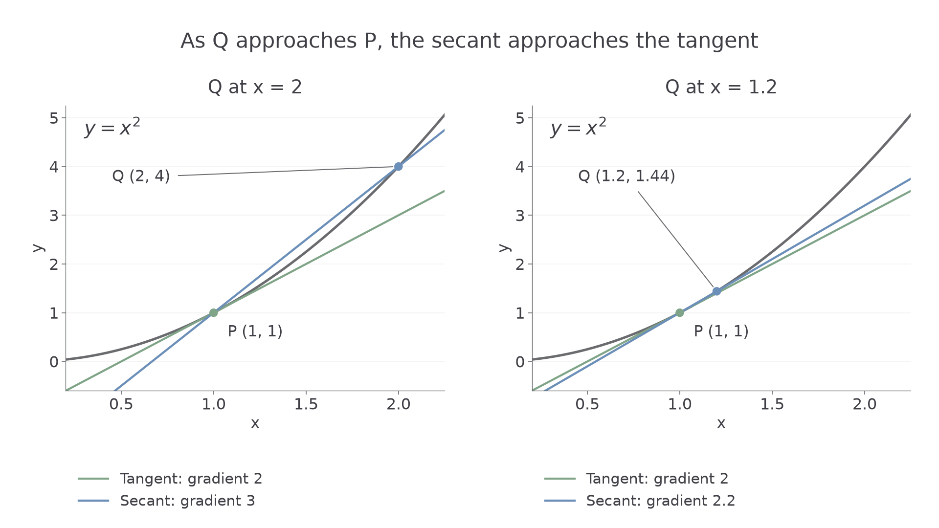
A line through two curve points is a secant. Keep the first point fixed and move the second point closer. The secant approaches the tangent, the straight line with the curve's local direction. A tangent can cross the curve elsewhere; “touches once” is not its definition.

[DIAGRAM: asset_name: Secants approaching a tangent; asset_slug: secant-to-tangent; caption: Secants to y equals x squared approach the tangent at one comma one; description: Two panels show y equals x squared with P at one comma one. The left secant joins P to Q at two comma four and has gradient three. The right joins P to Q at one point two comma one point four four and has gradient two point two. Both panels include the tangent y equals two x minus one, with gradient two.]
Secants to y equals x squared approach the tangent at one comma one

Derivative

The derivative of $y=f(x)$ , written $f'(x)$ or $\dfrac{dy}{dx}$ , gives the tangent gradient at each input where that gradient exists. Finding it is called differentiation. At $x=a$ , the particular gradient is $f'(a)$ .

The symbol $dy/dx$ is derivative notation, not an instruction to divide the ordinary coordinates $y$ and $x$ . A derivative need not exist at every point: for example, the sharp corner of $y=|x|$ at zero has no single tangent gradient. Our rules will be used where the function has a finite derivative.

Worked example 1: approaching a positive gradient

Question. Estimate the tangent gradient to $y=x^2$ at $(1,1)$ using nearby points with $x=1.1$ and $x=0.9$ .

Plan. Calculate the two secant gradients using rise divided by run.

m_{\text{right}}=\frac{1.21-1}{1.1-1}=2.1, \qquad m_{\text{left}}=\frac{0.81-1}{0.9-1}=1.9.

Closer points at $1.01$ and $0.99$ give $2.01$ and $1.99$ . The gradients approach $2$ .

Answer. The tangent gradient is estimated as $2$ ; the power rule below will give $f'(1)=2$ exactly.

Check. The line $y=2x-1$ passes through $(1,1)$ . Its vertical difference from the curve is $x^2-(2x-1)=(x-1)^2$ , very small near $x=1$ , consistent with the pictured tangent.

Reflecting the curve in the horizontal axis reverses the rises while keeping the same runs.

Worked example 2: approaching a negative gradient

Question. Estimate the tangent gradient to $y=-x^2$ at $(1,-1)$ , again using $x=1.1$ and $x=0.9$ .

Plan. Use the new curve heights and retain the signs of both differences.

m_{\text{right}}=\frac{-1.21-(-1)}{1.1-1}=-2.1, \qquad m_{\text{left}}=\frac{-0.81-(-1)}{0.9-1}=-1.9.

At $1.01$ and $0.99$ , the corresponding gradients are $-2.01$ and $-1.99$ .

Answer. The tangent gradient is estimated as $-2$ .

Check. The curve falls as $x$ increases near $1$ , so the gradient must be negative. Reflection of the first curve changes its tangent gradient from $2$ to $-2$ .

Nearby-point calculations explain the meaning; a formal limiting proof is not needed to use the differentiation rules. Check that meaning before calculating algebraically.

Differentiating powers

A rule can replace repeated nearby-point calculations. For $y=x^2$ , it gives $dy/dx=2x$ : the gradient is $2$ at $x=1$ , $6$ at $x=3$ , and changes continuously between them.

Power rule

\frac{d}{dx}(x^n)=nx^{n-1}.

Multiply by the old power, then subtract $1$ from that power. Apply the rule at inputs where the real function and its derivative are defined.

This standard derivative must be learnt; it is not on the provided formulae sheet.

The exponent can be negative or fractional. Rewrite carefully: $1/x^2=x^{-2}$ , $\sqrt{x}=x^{1/2}$ , and $1/\sqrt{x}=x^{-1/2}$ . The first requires $x\ne0$ ; the last requires $x>0$ . Although $\sqrt{x}$ exists at zero, its derivative $1/(2\sqrt{x})$ does not have a finite value there. For fractional powers, work within a real interval on which the power and derivative are defined; $x>0$ always avoids the fractional-power boundary issues used here.

Worked example 3: a positive integer power

Question. Differentiate $f(x)=x^5$ .

Plan. Multiply by $5$ and reduce the exponent to $4$ .

f'(x)=5x^{5-1}=5x^4.

Answer. $f'(x)=5x^4$ , for all real $x$ .

Check. Near $x=1$ , the secant from $1$ to $1.001$ has gradient $(1.001^5-1)/0.001\approx5.010$ , close to $f'(1)=5$ .

The next exponent is negative and fractional. Subtracting $1$ makes it more negative.

Worked example 4: a reciprocal square root

Question. Differentiate $g(x)=1/\sqrt{x}$ , for $x>0$ .

Plan. Rewrite as $x^{-1/2}$ , then apply the same power rule.

g(x)=x^{-1/2}, \qquad g'(x)=-\frac12x^{-1/2-1}=-\frac12x^{-3/2}=-\frac{1}{2x^{3/2}}.

Answer. $g'(x)=-1/(2x^{3/2})$ , for $x>0$ .

Check. At $x=4$ the derivative is $-1/16$ . The nearby-point gradient $(1/\sqrt{4.001}-1/2)/0.001\approx-0.062488$ , close to $-0.0625$ . Its negative sign matches the decreasing reciprocal root.

Last Accessed

Number

Algebra

Series

Geometry

Trigonometry

Calculus

9A - Gradients and the power rule

Gradient at a point

Differentiating powers

Continue this lesson.

Learn faster with Nova