4.6.1.1 - Measuring rates and interpreting rate graphs

Mean rate and its units

Mean rate compares the amount of chemical change with the time taken for that change.

Measure a quantity that changes because of the reaction. A gas syringe can measure the volume of gaseous product in $\mathrm{cm^3}$. A balance can measure a decrease in the apparatus mass when a gaseous product escapes; that mass loss measures the escaped product, not disappearance of all matter. Reactants can also be measured directly where an appropriate method is available. Temperature change alone is not a quantity of reactant used or product formed.

Worked example 1 — gas volume

A reaction produces $48\,\mathrm{cm^3}$ of gas in $40\,\mathrm{s}$. Divide product volume by elapsed time:

Multiplying back, $1.2\times40=48\,\mathrm{cm^3}$, checks that the result describes the measured amount.

Worked example 2 — mass and a time conversion

Another reaction uses $0.84\,\mathrm{g}$ of reactant in 2 minutes. Convert the time before calculating a per-second rate:

The unit follows the measured quantity: mass gives $\mathrm{g/s}$, volume gives $\mathrm{cm^3/s}$. Dividing by 2 would give grams per minute rather than grams per second.

For an interval after the reaction has started, use changes in quantity and time. If gas volume rises from $12$ to $36\,\mathrm{cm^3}$ between $10$ and $30\,\mathrm{s}$, the interval mean is $(36-12)/(30-10)=1.2\,\mathrm{cm^3/s}$. Dividing 36 by 30 would give the mean from the start if the initial volume were zero, not the requested interval mean.

Mean rate hides changes within its interval. A reaction can be fast initially and slow later while still having one mean for the entire run. Compare measurements of the same quantity and reaction conditions; a gas-volume rate and a mass-loss rate cannot be compared by their numbers alone because their units and measured substances differ.

Drawing and reading quantity–time curves

A quantity–time curve shows both how much change has occurred and how its speed varies during a reaction.

Put time on the horizontal axis and the measured quantity on the vertical axis. Label units, choose regular scales, plot the data accurately and draw a suitable smooth best-fit curve. Do not force a curve through an anomalous point or join each point with a sharp zigzag unless the data justify straight segments.

These illustrative gas-production data describe a smooth reaction model:

The product curve starts at zero, rises rapidly, becomes less steep and finally levels off at $60\,\mathrm{cm^3}$. Its height tells you the accumulated product, while its slope tells you the rate. At $80\,\mathrm{s}$ there is more product than at $20\,\mathrm{s}$, but production is slower because the curve is flatter.

[DIAGRAM: asset_name: Product formed and reactant remaining; asset_slug: 8462_c41_quantity_curves; caption: Product accumulates while reactant is used; both curves flatten as the reaction stops.; description: Two illustrative smooth quantity–time graphs on matching time axes from 0 to 140 seconds. The left graph shows gas produced rising from 0 to 60 cm³ by 100 seconds and then remaining constant, with the table's points. The right shows a measured reactant mass decreasing from 1.0 g to 0.4 g over the same time and then remaining constant. These are separate measured quantities, not directly subtractable units.]

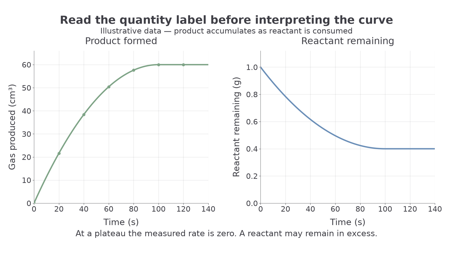
A graph of reactant used up also rises from zero because cumulative consumption increases. A graph of reactant remaining falls instead. A mass-of-apparatus graph falls when product gas escapes, whereas a mass-of-gas-produced graph rises. Read the axis label before deciding what a rising or falling curve means.

Flattening indicates no further measured chemical change. A reactant may have been used up, leaving another reactant in excess, so a remaining-reactant curve need not reach zero. Equal final gas volumes in two runs, under the same collection conditions, indicate equal final amounts of that gaseous product. A steeper curve reaching the same plateau sooner indicates a faster reaction producing the same final amount.

Optional notebook construction — ungraded. Plot the gas-volume table, label both axes and draw the smooth curve. Check the coordinate $(40,38.4)$, the falling steepness, and the horizontal plateau after $100\,\mathrm{s}$ against the left panel.

Slopes, tangents and reaction speed

The slope of a quantity–time curve measures how quickly that quantity is changing at a particular stage.

A steep upward product curve indicates rapid product formation. A steep downward remaining-reactant curve indicates rapid reactant consumption. Compare the magnitude of the slopes for speed: a downward slope has a negative sign, but reactant-use rate is normally reported as a positive quantity. A horizontal curve has zero slope and no further measured change.