4.3.1.4 - Chemical measurements and uncertainty
Learn why every chemical measurement has uncertainty and how repeated results, their mean and their spread help describe it. Distinguish random variation from consistent bias, then use that distinction to choose improvements that make evidence more useful.
Resolution and measurement uncertainty
A measuring instrument gives a reading with limited detail, so a reported value cannot be treated as perfectly exact.
Resolution is the smallest change that an instrument can display or distinguish. A digital balance reading to 0.01 g cannot show a difference of 0.001 g. An analogue measuring cylinder with marks every allows only limited judgement of a liquid level between marks. Read the bottom of the meniscus at eye level for a clear liquid, with the cylinder upright on a level surface, to avoid parallax.
Uncertainty describes doubt about a measurement. Instrument resolution is one source; judgement of an end point, fluctuating readings and variation in the method can also matter. Recording many decimal places after a calculation does not remove the uncertainty of the measurements used.
For an analogue scale that permits judgement between divisions, one estimate of reading uncertainty is half the smallest division. Applying that convention to a cylinder divided every :
For a thermometer marked every :
These estimates concern reading the scales. End-point judgement and other method effects can contribute additional uncertainty. Use any instrument uncertainty supplied in a task; a digital instrument's stated uncertainty can differ from its resolution.
Choose apparatus appropriate to the quantity. A measuring cylinder is suitable for an approximate volume; a volumetric pipette delivers a particular volume more precisely. A balance should have sufficient resolution for the change in mass expected. If a change is only 0.02 g, a balance resolving 0.1 g cannot distinguish it reliably.
Means, ranges and distributions
Repeated measurements reveal how results are distributed rather than leaving us dependent on one reading.
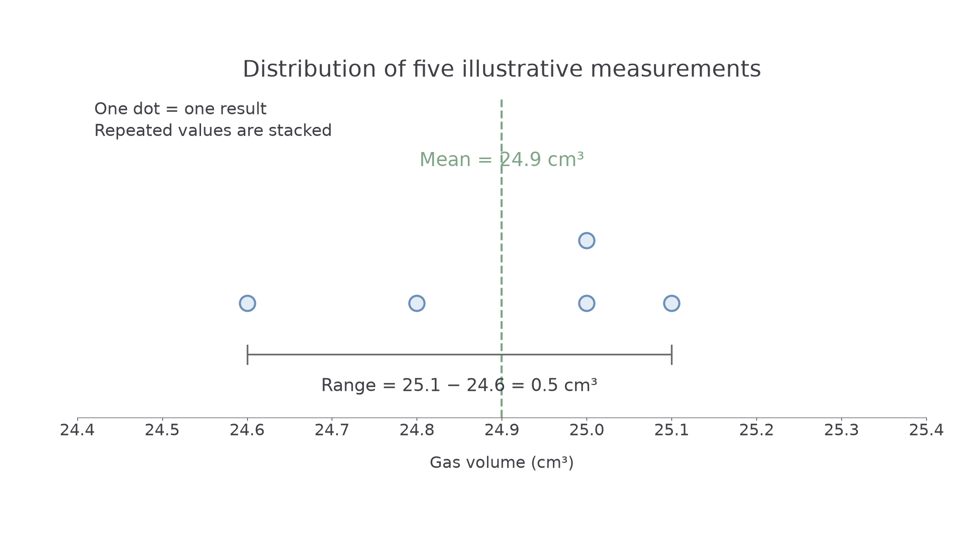
In an Illustrative experiment, five measurements of gas volume are 24.6, 24.8, 25.0, 25.0 and . The mean is their sum divided by the number of measurements:
The range is the maximum minus the minimum, so . It measures spread. The observations extend from below the mean to above it. Keeping that interval communicates the actual observed spread.
One commonly stated estimate of uncertainty from repeats is half the range, here . A report might use mean , estimated uncertainty , explicitly saying the estimate is half the range. It does not assert that the unknown true value must lie there. The mean need not be exactly halfway between the extreme observations, and the estimate does not detect systematic errors. Follow the uncertainty convention specified in the task.
Illustrative timing data: three valid measurements are 62, 65 and 63 s. Calculate their centre and spread separately:
The mean uses every valid reading, whereas the range uses the extremes. A shorter range would indicate less spread, without showing whether the timer had a consistent offset.
A dot plot places each measurement on a common scale, stacking dots where values repeat. A frequency table counts how often each value or interval occurs. For many measurements, grouped frequencies can show whether results cluster tightly or are widely spread. Keep the units and interval boundaries clear.
[DIAGRAM: asset_name: Repeated volumes and their spread; asset_slug: 8462_c19_result_distribution; caption: The five illustrative gas-volume results cluster around a mean of 24.9 cubic centimetres and span a range of 0.5 cubic centimetres.; description: Dot plot on a gas-volume axis from 24.4 to 25.4 cubic centimetres, with points at 24.6, 24.8, two stacked at 25.0 and one at 25.1. A dashed vertical line marks the mean 24.9; a horizontal bracket runs from 24.6 to 25.1 and is labelled range equals 0.5 cubic centimetres.]
Continue this lesson.
You’re previewing NovaLearn without an account. Create a free account to read the rest.
Create free account