9-11 - Kinematics Equations and Motion Graphs | Edexcel A-Level Physics

One-dimensional motion, the constant-acceleration equations, and displacement-time, velocity-time and acceleration-time graphs. You will connect the equations to the graph features so the symbols describe motion rather than replacing it.

Motion Along One Line

Imagine a trolley moving along a straight track. You choose one direction as positive, perhaps to the right along the track. From that moment, every velocity, acceleration and displacement in the problem is described relative to that choice.

For this lesson, the motion is one-dimensional. That means the object can move forwards or backwards along the same line, but we are not resolving vectors at angles or treating projectiles yet.

The five quantities used in uniformly accelerated motion are:

Symbol	Meaning	SI unit
$s$	displacement from the starting position	$\mathrm{m}$
$u$	initial velocity	$\mathrm{m\,s^{-1}}$
$v$	final velocity	$\mathrm{m\,s^{-1}}$
$a$	acceleration, the rate of change of velocity	$\mathrm{m\,s^{-2}}$
$t$	time taken	$\mathrm{s}$

Displacement

The distance moved in a stated direction from a starting position; a vector, so it can be negative along a line.

The word "displacement" matters. If the trolley starts at a mark, travels forwards, then comes back past the mark, its displacement can be negative even though the distance it has travelled is positive. In one-dimensional kinematics, the sign is part of the physical information.

Uniform acceleration

Acceleration that is constant: the velocity changes by the same amount in each equal time interval.

Uniform acceleration does not mean the velocity is constant. A car whose velocity changes from $4\,\mathrm{m\,s^{-1}}$ to $6\,\mathrm{m\,s^{-1}}$ to $8\,\mathrm{m\,s^{-1}}$ in equal one-second intervals has uniform acceleration. A car travelling at $8\,\mathrm{m\,s^{-1}}$ all the time has zero acceleration.

A common trap is to read a negative acceleration as "the object is slowing down". That is only sometimes true. Negative acceleration means acceleration in the negative chosen direction. If an object is moving in the negative direction and has negative acceleration, it is speeding up.

Edexcel supplies the main kinematic equations in the data/formulae booklet. The assessed skill is not memorising a list; it is deciding whether the model fits and which quantities belong in the equation.

Equations From a Velocity-Time Graph

The cleanest way to understand the constant-acceleration equations is to start with a velocity-time graph.

If acceleration is uniform, the velocity-time graph is a straight line. Its gradient is acceleration:

\begin{aligned} \text{acceleration} &= \text{change in velocity}/ \text{time taken} \\ a &= \frac{v - u}{t} \end{aligned}

Rearranging gives:

v = u + at

The area under a velocity-time graph gives displacement. For a straight-line velocity-time graph, that area is a trapezium. Its two parallel sides are $u$ and $v$ , and its width is $t$ , so:

s = \frac{(u + v)t}{2}

The same graph also gives the two other supplied equations. Since $v = u + at$ , the average velocity during uniform acceleration is halfway between $u$ and $v$ :

\text{average velocity}= \frac{u + v}{2} = u + \frac{1}{2}at

Multiplying by time:

s = ut + \frac{1}{2}at^{2}

Combining $v = u + at$ with the area idea gives:

v^{2} = u^{2} + 2as

The equations are not four separate tricks. They are different ways of reading the same straight velocity-time graph.

Equations for uniformly accelerated motion

v = u + at \qquad s = \frac{(u + v)t}{2} \qquad s = ut + \frac{1}{2}at^{2} \qquad v^{2} = u^{2} + 2as

$s$ : displacement (m); $u$ , $v$ : initial and final velocity (m s⁻¹); $a$ : acceleration (m s⁻²); $t$ : time (s). Valid only for constant acceleration along a straight line; choose a positive direction and keep signs.

Worked example: a small test vehicle moves in a straight line. Its velocity increases uniformly from $4.0\,\mathrm{m\,s^{-1}}$ to $16.0\,\mathrm{m\,s^{-1}}$ in $6.0\,\mathrm{s}$ . Find its acceleration and displacement.

Decision point 1: can we use constant-acceleration equations? Yes, the question says the velocity increases uniformly.

Decision point 2: what does the graph say? A straight velocity-time line has gradient equal to acceleration and area equal to displacement.

Acceleration:

\begin{aligned} a &= \frac{v - u}{t} \\ a &= \frac{16.0 - 4.0}{6.0} \\ a &= 2.0\,\mathrm{m\,s^{-2}} \end{aligned}

Displacement:

\begin{aligned} s &= \frac{(u + v)t}{2} \\ s &= \frac{(4.0 + 16.0) \times 6.0}{2} \\ s &= 60\,\mathrm{m} \end{aligned}

The units check the representation: velocity multiplied by time gives $\mathrm{m\,s^{-1}} \times \mathrm{s} = \mathrm{m}$ , so the area really is a displacement.

Choosing the Right Equation

When a kinematics question gives numbers, resist the urge to grab the first equation that contains the unknown. Start with a short decision route.

Choose and state the positive direction if signs matter.
Write the known quantities with units.
Check that acceleration is uniform before using SUVAT across the interval.
Identify the unknown and the missing quantity.
Choose the equation that leaves out the missing quantity.

Equation	Useful when the missing quantity is...
$s = ((u + v)t)/2$	$a$
$v = u + at$	$s$
$s = ut + \frac{1}{2}at^{2}$	$v$
$v^{2} = u^{2} + 2as$	$t$

Worked example: a cyclist travels in the positive direction at $12.0\,\mathrm{m\,s^{-1}}$ and brakes uniformly to rest over a displacement of $36.0\,\mathrm{m}$ . Calculate the acceleration and the stopping time.

Knowns:

\begin{aligned} u &= +12.0\,\mathrm{m\,s^{-1}} \\ v &= 0 \\ s &= +36.0\,\mathrm{m} \\ a &= ? \\ t &= ? \end{aligned}

Decision point 1: time is not given, so start with the equation that leaves out $t$ .

\begin{aligned} v^{2} &= u^{2} + 2as \\ 0^{2} &= 12.0^{2} + 2a(36.0) \\ 0 &= 144 + 72a \\ a &= -2.00\,\mathrm{m\,s^{-2}} \end{aligned}

Decision point 2: the negative sign is not a mistake. The cyclist is moving in the positive direction, but the acceleration is in the negative direction, so the cyclist slows down.

Now use an equation that contains $t$ :

\begin{aligned} v &= u + at \\ 0 &= 12.0 + (-2.00)t \\ t &= 6.00\,\mathrm{s} \end{aligned}

For an ordinary Edexcel “calculate” question, a correct final value can earn the applicable calculation marks without written working. Showing the relationship and substitution makes partial method credit possible if a later result is wrong; an explicitly requested derivation or explanation still needs that evidence. For “show that”, keep one extra significant figure in your working before rounding to the stated value.

Reading Motion Graphs

Each motion graph has a different job. A strong interpretation starts by asking: is this graph telling me a slope story or an area story?

[DIAGRAM: asset_name: Linked displacement, velocity and acceleration graphs; asset_slug: 9ph0_motion_graphs; recommended_method: deterministic; description: Displacement, velocity and acceleration against time for acceleration from rest at 3 m s⁻² for 4 s followed by 3 s at 12 m s⁻¹. Velocity graph areas are 24 m and 36 m.]
Diagram

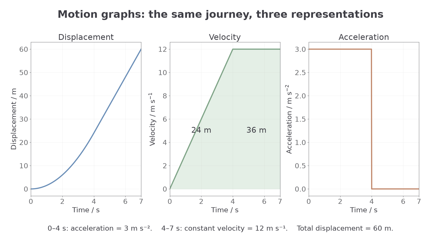
On a displacement-time graph:

the gradient gives velocity
a steeper positive gradient means a larger positive velocity
a horizontal section means zero velocity
a negative gradient means velocity in the negative direction
a tangent to a curve gives instantaneous velocity at that time

The tempting mistake is to say that a steeper displacement-time graph means greater acceleration. It does not. The slope of a displacement-time graph is velocity. Acceleration appears only when that slope is changing.

On a velocity-time graph:

the gradient gives acceleration
the area between the graph and the time axis gives displacement
an intercept on the velocity axis gives the initial velocity
area below the time axis counts as negative displacement

On an acceleration-time graph:

the area between the graph and the time axis gives change in velocity
a horizontal line above zero means constant positive acceleration
a line on zero means constant velocity, not necessarily zero velocity

Gradient of displacement–time = velocity; gradient of velocity–time = acceleration; area under velocity–time = displacement; area under acceleration–time = change in velocity.

Another useful contrast: area under a velocity-time graph has units $\mathrm{m\,s^{-1}} \times \mathrm{s} = \mathrm{m}$ , so it is displacement. Area under an acceleration-time graph has units $\mathrm{m\,s^{-2}} \times \mathrm{s} = \mathrm{m\,s^{-1}}$ , so it is change in velocity. Area under a displacement-time graph gives $\mathrm{m\,s}$ , which is not one of the standard kinematic quantities in this course.

Worked example: a velocity-time graph for a trolley starts at $v = 0$ when $t = 0$ , rises in a straight line to $12\,\mathrm{m\,s^{-1}}$ at $t = 4.0\,\mathrm{s}$ , then stays at $12\,\mathrm{m\,s^{-1}}$ until $t = 7.0\,\mathrm{s}$ .

From $0$ to $4.0\,\mathrm{s}$ , the gradient is:

a = \frac{12 - 0}{4.0} = 3.0\,\mathrm{m\,s^{-2}}

The displacement from $0$ to $4.0\,\mathrm{s}$ is the triangular area:

s = \frac{1}{2} \times 4.0 \times 12 = 24\,\mathrm{m}

The displacement from $4.0\,\mathrm{s}$ to $7.0\,\mathrm{s}$ is the rectangular area:

s = 3.0 \times 12 = 36\,\mathrm{m}

Total displacement:

24\,\mathrm{m} + 36\,\mathrm{m} = 60\,\mathrm{m}

For an Edexcel “interpret” question, do not just name the graph feature. Translate it into the physical quantity: "the gradient is positive and constant, so the acceleration is positive and constant."

For total distance, add the magnitudes of the areas above and below the time axis. For example, areas $+9\,\mathrm m$ and $-3\,\mathrm m$ give displacement $+6\,\mathrm m$ but distance $12\,\mathrm m$ . Split an interval at each zero crossing before calculating distance. The slope of an acceleration–time graph is the rate of change of acceleration; it is not velocity or displacement.

Non-Uniform Motion

The constant-acceleration equations only describe an interval where acceleration is uniform. If a velocity-time graph is curved, the acceleration is changing, so using one SUVAT equation across the whole curve is usually the wrong model.

[DIAGRAM: asset_name: Instantaneous acceleration from a tangent; asset_slug: 9ph0_tangent_gradient; recommended_method: deterministic; description: Curved velocity-time graph v=t²+t with tangent at 2 s and a large gradient triangle giving instantaneous acceleration 5 m s⁻²; whole-interval average is 4 m s⁻².]
Diagram

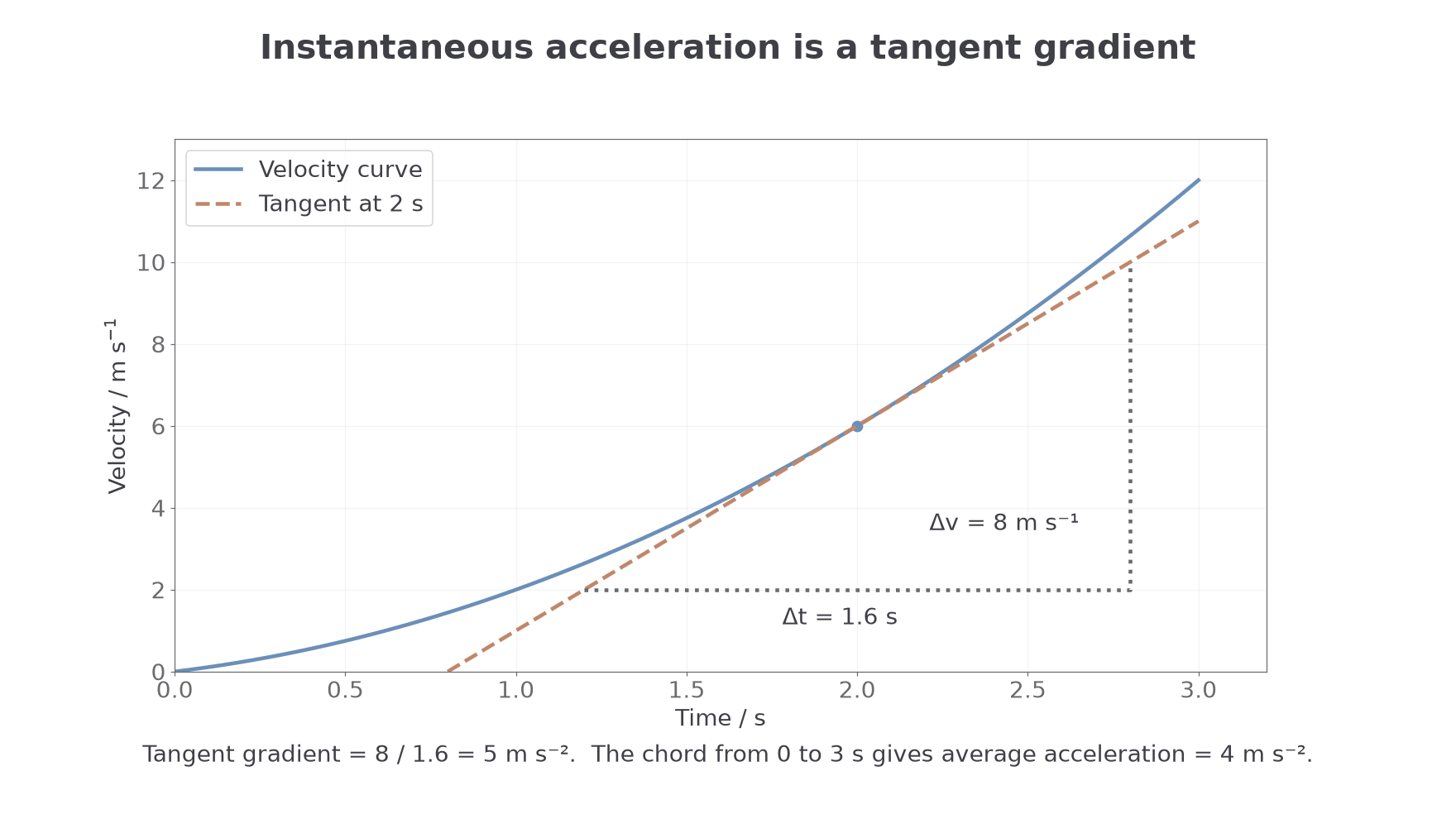
For non-uniform motion, graph methods become the safer language.

On a curved displacement-time graph:

average velocity over an interval is the gradient of the chord joining the two endpoints
instantaneous velocity at one time is the gradient of the tangent at that time

On a curved velocity-time graph:

average acceleration over an interval is the gradient of the chord joining the two endpoints
instantaneous acceleration at one time is the gradient of the tangent at that time
displacement is still the area under the graph, often estimated using trapezia or counting squares

On any acceleration-time graph:

the area under the graph still gives change in velocity, even if acceleration is not constant

Worked example: a motion sensor gives these velocity readings for a toy car.

$t$ / s	0	1	2	3
$v$ / m s⁻¹	0	2	6	12

The velocity is not increasing by the same amount each second: $+2$ , then $+4$ , then $+6\,\mathrm{m\,s^{-1}}$ . The acceleration is not uniform, so a single SUVAT calculation across $0$ to $3\,\mathrm{s}$ is not justified.

Estimate the displacement from the area under the velocity-time data using trapezia:

\begin{aligned} 0\text{ to }1\,\mathrm{s}: \frac{(0 + 2) \times 1}{2} &= 1\,\mathrm{m} \\ 1\text{ to }2\,\mathrm{s}: \frac{(2 + 6) \times 1}{2} &= 4\,\mathrm{m} \\ 2\text{ to }3\,\mathrm{s}: \frac{(6 + 12) \times 1}{2} &= 9\,\mathrm{m} \\ \text{total displacement} &= 14\,\mathrm{m} \end{aligned}

The average acceleration over the whole $3\,\mathrm{s}$ is:

\text{average acceleration}= \frac{12 - 0}{3} = 4\,\mathrm{m\,s^{-2}}

That average acceleration is useful, but it is not the same as saying the acceleration was $4\,\mathrm{m\,s^{-2}}$ at every instant. If you wrongly used $s = ut + \frac{1}{2}at^{2}$ with $a = 4\,\mathrm{m\,s^{-2}}$ , you would get $18\,\mathrm{m}$ , not the graph estimate of $14\,\mathrm{m}$ . The difference is the warning sign: the constant-acceleration model did not fit the data.

In practical or Paper 3 style contexts, the graph is only as trustworthy as the data. A data logger or motion sensor can reduce reaction-time uncertainty and take many readings quickly, but you still need sensible axes, units, a best-fit line or curve where appropriate, and a justified tangent for an instantaneous gradient. Calculate its gradient using widely separated points on the tangent, so the same reading uncertainty is a smaller fraction of the rise and run. Scatter about a trend suggests random uncertainty; a straight-line graph that should pass through the origin but does not may suggest a systematic error, such as an offset in the sensor.

Braking and Constructing Motion Graphs

A graph sketch must preserve how the physical quantities are related. For uniform braking, draw a straight velocity–time line down to zero, a constant negative acceleration–time line during braking, and a displacement–time curve whose positive gradient decreases to zero. After the object stops and remains stationary, velocity and acceleration are zero while displacement is constant. A negative acceleration does not mean the displacement–time curve slopes down while the object still moves forwards.

Use labelled axes and units. For a quantitative plot choose a scale that spreads the data over the available space, then plot accurate points. Use a straight best-fit line only when the model predicts a linear relationship; use a smooth curve for changing acceleration. A sketch shows correct shape and intercepts even when no numerical scale is requested.

Worked braking example: A car moving at $22.0\,\mathrm{m\,s^{-1}}$ brakes uniformly to rest with acceleration $-7.8\,\mathrm{m\,s^{-2}}$ . Show that the stopping displacement is about $31\,\mathrm{m}$ .

Decision point 1: choose the positive direction as the car's initial motion.

\begin{aligned} u &= +22.0\,\mathrm{m\,s^{-1}} \\ v &= 0 \\ a &= -7.8\,\mathrm{m\,s^{-2}} \\ s &= ? \end{aligned}

Decision point 2: time is missing, so use:

v^{2} = u^{2} + 2as

Substitute signed values:

\begin{aligned} 0^{2} &= 22.0^{2} + 2(-7.8)s \\ 0 &= 484 - 15.6s \\ s &= \frac{484}{15.6} \\ s &= 31.0256\ldots \,\mathrm{m} \end{aligned}

So the stopping displacement is $31\,\mathrm{m}$ to two significant figures. The negative acceleration and positive displacement can coexist: the car is still moving forwards while its velocity is being reduced.

The same situation on a velocity-time graph would be a straight line sloping down to zero. The gradient is negative acceleration; the triangular area under the graph is positive displacement.

Last Accessed

Topic 1: Working as a Physicist

Topic 2: Mechanics

Topic 3: Electric Circuits

Topic 4: Materials

Topic 5: Waves and Particle Nature of Light

Topic 6: Further Mechanics

Topic 7: Electric and Magnetic Fields

Topic 8: Nuclear and Particle Physics

Topic 9: Thermodynamics

Topic 10: Space

Topic 11: Nuclear Radiation

Topic 12: Gravitational Fields

Topic 13: Oscillations

9-11 - Kinematics Equations and Motion Graphs