181-183 - Simple Harmonic Motion Equations and Periods

The restoring-force condition

Picture a trolley attached to a light spring on a smooth track. If the trolley is pulled to the right and released, the spring pulls it back left. If the trolley is pushed to the left, the spring pushes it back right. The important feature is not just that the trolley moves to and fro; it is that the force always tries to restore the trolley to its equilibrium position.

Take the equilibrium position as $x = 0$. Displacement $x$ is measured from that point, with a sign:

• $x > 0$ means displacement to the right.
• $x < 0$ means displacement to the left.
• $x = 0$ means the object is at equilibrium.

For simple harmonic motion, the resultant force must be proportional to displacement and opposite in direction:

$F$ is the resultant force in $\mathrm{N}$, $x$ is displacement from equilibrium in $\mathrm{m}$, and $k$ is the proportionality constant in $\mathrm{N\,m^{-1}}$. For a spring, $k$ is the spring constant. In another oscillator, the same form may come from a different physical source.

[DIAGRAM: asset_name: Three horizontal spring states with aligned equilibrium reference, x=-A,0,+A and inward restoring force arrows; asset_slug: 053_simple_harmonic_motion_equations_periods__diagram_01; recommended_method: matplotlib; description: Three horizontal spring states with aligned equilibrium reference, x=-A,0,+A and inward restoring force arrows.]

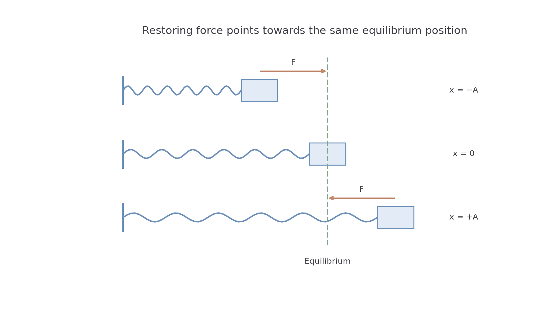
The minus sign is directional. If $x$ is positive, $F$ is negative. If $x$ is negative, $F$ is positive. At equilibrium, $x = 0$, so the restoring force is zero.

This gives a useful way to identify SHM:

• A straight-line force-displacement graph through the origin can indicate SHM.
• The gradient must be negative if positive displacement is taken in the positive direction.
• The force must be the resultant restoring force, not just one force among several.

A small-angle simple pendulum can also fit the model because the tangential component of weight is approximately proportional to displacement and directed back towards the centre. A large-angle pendulum does not fit exactly because the restoring force is no longer proportional to displacement.

Misconception contrast: moving backwards and forwards is not enough for SHM. A bouncing ball moves up and down, but during contact the force is not a smooth $-kx$ restoring force for the whole motion. SHM needs the proportional restoring-force condition.

For a vertical spring, measure $x$ from the loaded equilibrium position. Weight and the equilibrium spring force cancel; the additional resultant restoring force is $-kx$. The extension from the unstretched length is not the SHM displacement. Peak-to-peak displacement is $2A$.

From force to acceleration

Newton's second law links the restoring force to acceleration:

Combine this with the SHM condition:

The constant $k/m$ has units $\mathrm{s^{-2}}$. In SHM it is written as $\omega^{2}$, so:

$\omega$ is the angular frequency in $\mathrm{rad\,s^{-1}}$. The radian is dimensionless, but writing $\mathrm{rad\,s^{-1}}$ helps distinguish angular frequency from ordinary frequency.

The physical meaning is sharp:

• acceleration is proportional to displacement from equilibrium
• acceleration is in the opposite direction to displacement
• acceleration is zero at equilibrium
• acceleration has its greatest magnitude at the extremes

Worked example: a $0.150\,\mathrm{kg}$ glider is attached to a spring of spring constant $6.0\,\mathrm{N\,m^{-1}}$. At one instant the glider is $0.040\,\mathrm{m}$ to the right of equilibrium. Calculate the restoring force and acceleration.

The sign convention is the first decision. Take right as positive, so $x = +0.040\,\mathrm{m}$.

The negative sign means the force acts left, back towards equilibrium.

The acceleration also acts left. You can reach the same result through $a = -\omega^{2} x$:

For “calculate”, Edexcel-style credit usually sits in the equation, substitution, numerical answer and unit. The sign should be explained if direction matters.

Using the time equations

The SHM equations in the specification describe an oscillator when time is measured from the instant it is at its positive maximum displacement. That starting choice makes:

$A$ is the amplitude in $\mathrm{m}$: the maximum displacement from equilibrium. $t$ is time in $\mathrm{s}$. $v$ is velocity in $\mathrm{m\,s^{-1}}$. $a$ is acceleration in $\mathrm{m\,s^{-2}}$.

The equations tell one consistent story. At $t = 0$:

The oscillator is at its positive extreme, momentarily at rest, accelerating back towards equilibrium.

The acceleration equation also links back to the SHM condition: