58 - Elastic Strain Energy
Elastic strain energy stored during stretching. The key move is to read work from the force-extension graph, so the area under the graph becomes a physical energy transfer.
Work Stored in the Stretch
Pull an elastic cord slowly. At the start, the cord hardly pulls back. As the extension grows, the force you must apply grows. That means the work done is not usually found by multiplying the final force by the final extension, because the force was not that large for the whole stretch.
The useful picture is a force-extension graph:
- the vertical axis is force, , in newtons, N
- the horizontal axis is extension, , in metres, m
- the area under the graph has units N m, which is the same as joules, J
Elastic strain energy
The energy stored in a deformed material that is released when it returns to its original shape; equal to the work done in deforming it elastically.
So the area under a force-extension graph gives the work done in deforming the sample. If the deformation is elastic and the sample returns along the same path when unloaded, that work is stored as elastic strain energy. If the material is stretched beyond elastic behaviour, the loading area still represents work done, but not all of it may be recoverable as elastic strain energy.
The key contrast is:
- is work done by a constant force through distance .
- Area under the against graph is work done when the force changes during the stretch.
Straight-Line Graphs
For a sample that gives a straight force-extension graph through the origin, the area under the graph is a triangle. The triangle has:
- height , the final force at the final extension
- base , the final extension
So
Elastic strain energy
: elastic strain energy (J); : final force (N); : extension (m). Only for a straight force-extension graph through the origin within the elastic region; otherwise use the area under the graph.
This is the Edexcel data-booklet relationship. The half is there because the force increases from to , so the average force during the stretch is .
Worked example:
A spring is stretched from its natural length to an extension of . The force-extension graph is a straight line through the origin, and the force at this extension is . Calculate the elastic strain energy stored.
Decision point 1: the graph is straight and through the origin, so the area is a triangle and is valid.
Decision point 2: extension must be in metres.
Interpretation: of work has been done stretching the spring. For elastic behaviour, that energy is stored and can be returned when the spring is released.
Misconception contrast: the answer is not . That calculation treats the force as if it were all the way through the stretch. The graph shows the force built up gradually.
Curved Graphs
A non-linear force-extension graph still stores the answer in its area. What changes is the shape of the area.
[DIAGRAM: asset_name: elastic graph areas; asset_slug: 9ph0_elastic_areas; recommended_method: matplotlib; description: Linear triangular work area compared with exact trapezium interpolation of the worked non-linear 0–8 cm data.]
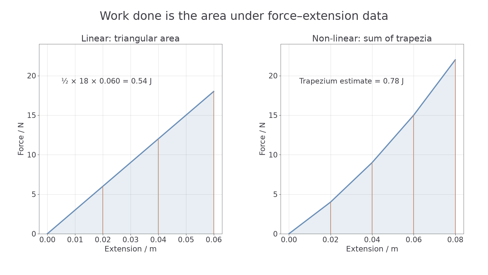
For a curved graph, do not automatically use . That formula assumes the area is a triangle. Instead, estimate the area under the curve by splitting it into strips, trapezia, rectangles, or graph-paper squares.
Worked example:
A rubber sample is stretched. The force and extension data are:
| Extension / cm | 0.0 | 2.0 | 4.0 | 6.0 | 8.0 |
|---|---|---|---|---|---|
| Force / N | 0.0 | 4.0 | 9.0 | 15.0 | 22.0 |
Determine the work done in stretching the sample from to .
Decision point 1: the force increases non-linearly, so use area under the data, not the triangle shortcut.
Decision point 2: the extension interval is .
Approximate each strip as a trapezium:
| Interval / cm | Mean force / N | Width / m | Area / J |
|---|---|---|---|
| 0.0 to 2.0 | 0.020 | 0.040 | |
| 2.0 to 4.0 | 0.020 | 0.130 | |
| 4.0 to 6.0 | 0.020 | 0.240 | |
| 6.0 to 8.0 | 0.020 | 0.370 |
Total area:
Continue this lesson.
You’re previewing NovaLearn without an account. Create a free account to read the rest.
Create free account