118-120 - Capacitor Charge, Discharge and Time Constant (CP11)

Why the Curve Flattens

Imagine a capacitor that has been charged to a p.d. $V_0$ and then connected across a resistor. At the start, the p.d. across the capacitor is large, so the electric field drives a relatively large current through the resistor. A moment later, some charge separation has been lost, the capacitor p.d. is smaller, and the current is smaller too.

That feedback is the reason for the curved graph. The capacitor is not losing the same p.d. every second. It loses the same fraction of what remains in equal time intervals, so the curve is steep at first and then gradually levels out towards zero.

For discharge through a fixed resistor, $Q$, $I$ and $V$ all follow the same exponential shape:

For charging from an initially uncharged capacitor through a fixed resistor, charge and p.d. rise from zero, steeply at first, towards their final values. After one time constant each has reached about $63\%$ of its final value. The charging current behaves differently: it starts at supply p.d./R and falls exponentially towards zero, reaching about $37\%$ of its initial magnitude after one time constant. To sketch these graphs, label time horizontally and Q, V or current magnitude vertically; show the correct start, changing gradient and limiting value. During discharge all three magnitudes fall exponentially from their initial values towards zero. Do not confuse the $37\%$ remaining on a falling curve with the $63\%$ gained on a rising charging curve.

Core Practical 11 Setup

Core Practical 11 asks you to display and analyse the p.d. across a capacitor as it charges and discharges through a resistor. The measuring instrument must be across the capacitor, because the variable you are analysing is $V$ across $C$, not the p.d. across the resistor.

[DIAGRAM: asset_name: Resistor-capacitor charge-discharge changeover circuit with voltage sensor across capacitor; asset_slug: 033_capacitor_discharge_time_constant_core_practical__diagram_01; recommended_method: matplotlib; description: Resistor-capacitor charge-discharge changeover circuit with voltage sensor across capacitor]

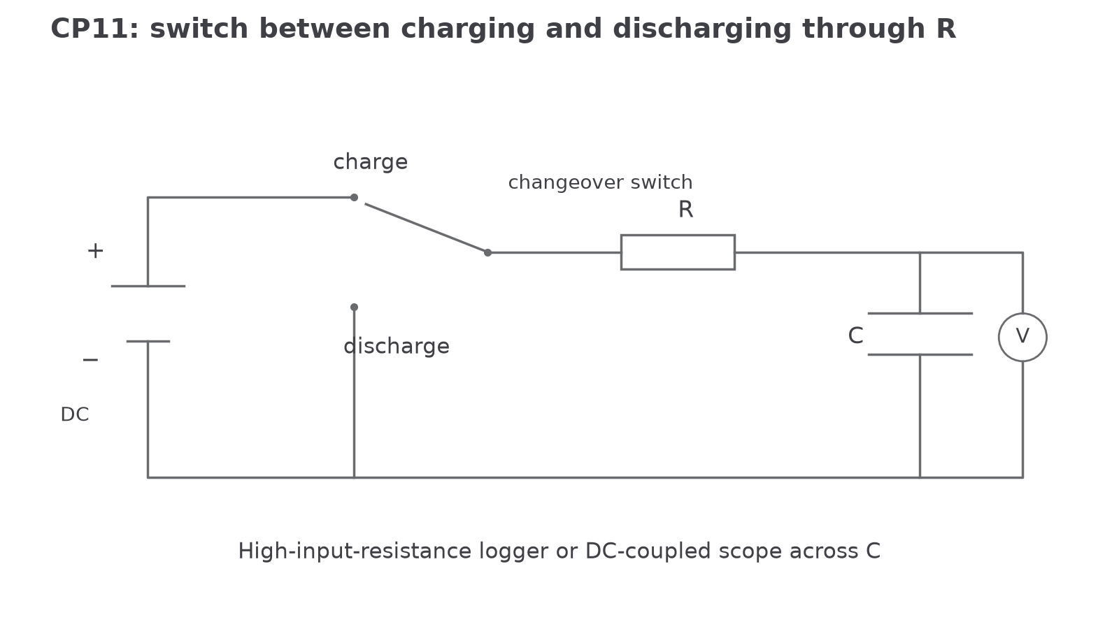
A practical route is:

1. Measure the resistance $R$ with a multimeter, rather than just trusting the colour bands.
2. Set a safe low DC supply p.d., below the capacitor voltage rating. Pearson's worksheet also states that open-circuit work should be below 40 V DC.
3. Connect the oscilloscope or data logger input in parallel with the capacitor.
4. Charge the capacitor and record the initial p.d. as $V_0$.
5. Start recording as the capacitor discharges through the resistor.
6. Use enough readings to analyse the shape: either a continuous data-logger trace, or repeated timings for the p.d. to fall to chosen values such as $5.0\,\mathrm{V}$, $4.0\,\mathrm{V}$, $3.5\,\mathrm{V}$.

The apparatus decision has a physics reason. A data logger can collect many $V, t$ pairs without reaction-time delay. An oscilloscope can show the shape directly if the time-base and volts-per-division settings are chosen so the trace uses the screen well. A handheld voltmeter and stopwatch can still work, but the first part of the discharge is fast, so timing and reading at the same instant becomes difficult.

Use a changeover switch: in the charge position, the supply, resistor and capacitor form a series loop; in the discharge position, isolate the supply and leave a closed resistor–capacitor loop. Record both transitions. Choose DC coupling on the oscilloscope so the actual capacitor p.d. and final level are retained. Set the time-base to show several time constants and trigger near the switching edge; with a logger, choose a sampling interval much smaller than $RC$. Start every repeat with the same fully charged initial p.d. An electrolytic capacitor must have the correct polarity and be discharged through a resistor before handling or changing the circuit.

Using the Exponential Model

The discharge equation is useful once you know $R$, $C$, $V_0$ and the time after discharge begins:

The decision point is the product $RC$. It is not a separate mystery constant; it is the resistance controlling the current multiplied by the capacitance that sets how much charge separation corresponds to a given p.d. Its unit is seconds:

Worked example:

A $220\,\mathrm{\mu F}$ capacitor is charged to $6.0\,\mathrm{V}$ and then discharged through a $47\,\mathrm{k\Omega}$ resistor. Calculate the p.d. across the capacitor after $15\,\mathrm{s}$.

Route:

Use the discharge equation because the capacitor has already been charged and is now losing p.d. through a resistor. Convert prefixes before finding $RC$.

Working: