39-41 - Resistivity and Charge Carriers (CP2) | Edexcel A-Level Physics

Using $R = \rho l / A$ , determining the electrical resistivity of a material in Core Practical 2, and using $I = nqvA$ to explain why materials have such different resistivities. The thread through the lesson is simple: first measure how a real wire resists current, then strip away its length and thickness to find the material property, then explain that property using moving charge carriers.

Resistance Comes From Shape and Material

Imagine two wires made from the same metal. One is long and thin; the other is short and thick. They are not equally easy routes for charge. A longer wire gives charge carriers more material to move through, so its resistance is larger. A thicker wire gives more parallel paths through the cross-section, so its resistance is smaller.

That physical story is written as

Resistance and resistivity

R = \frac{\rho l}{A}

$R$ : resistance (Ω); $\rho$ : resistivity of the material (Ω m); $l$ : length (m); $A$ : cross-sectional area (m²). For a uniform conductor at a stated temperature.

Resistivity

A property of a material, at a given temperature, equal to $RA/l$ for a uniform sample; unit Ω m.

Resistance belongs to a particular object. Resistivity belongs to the material, at a stated temperature. A short thick sample and a long thin sample of the same uniform material can have very different resistances, but they should give the same value of $\rho$ if measured well.

Rearrange the equation when the measurement is trying to find the material property:

\rho = \frac{RA}{l}

For a circular wire,

A = \pi r^{2} = \pi \frac{d^{2}}{4}

where $d$ is the diameter. The easy mistake is to put the diameter straight into $\pi r^{2}$ . Radius is half the diameter, and all distances in the area calculation must be in metres.

Worked example: from a wire measurement to resistivity

A uniform wire has length $0.800\,\mathrm{m}$ and diameter $0.240\,\mathrm{mm}$ . Its resistance is measured as $5.6\,\mathrm{\Omega}$ . Determine the resistivity of the wire material.

Decision point 1: the equation needs area, not diameter.

d = 0.240\,\mathrm{mm} = 2.40 \times 10^{-4}\,\mathrm{m}

r = \frac{d}{2} = 1.20 \times 10^{-4}\,\mathrm{m}

A = \pi r^{2} = \pi (1.20 \times 10^{-4})^{2} = 4.52 \times 10^{-8}\,\mathrm{m^{2}}

Decision point 2: use $\rho = RA/l$ , because the material property is the unknown.

\rho = (5.6)\frac{4.52 \times 10^{-8}}{0.800}

\rho = 3.2 \times 10^{-7}\,\mathrm{\Omega\,m}

Decision point 3: check the unit. $\mathrm{\Omega} \times \mathrm{m^{2}/m}$ leaves $\mathrm{\Omega\,m}$ , which is the unit of resistivity.

Misconception contrast: saying "this material has a resistance of $5.6\,\mathrm{\Omega}$ " is not precise. That value belongs to this particular length and thickness. The material has a resistivity of about $3.2 \times 10^{-7}\,\mathrm{\Omega\,m}$ under these conditions.

Core Practical 2 Method

Core Practical 2 determines the electrical resistivity of a material, commonly using a long piece of constantan wire fixed along a metre ruler.

[DIAGRAM: asset_name: CP2 resistivity apparatus and gradient; asset_slug: 9ph0_cp2_resistivity; recommended_method: deterministic; description: Unpowered wire on a metre rule measured between fixed and movable contacts by an ohmmeter. R against l graph has a positive constant lead/contact intercept and gradient rho/A; area uses micrometer diameter.]
Diagram

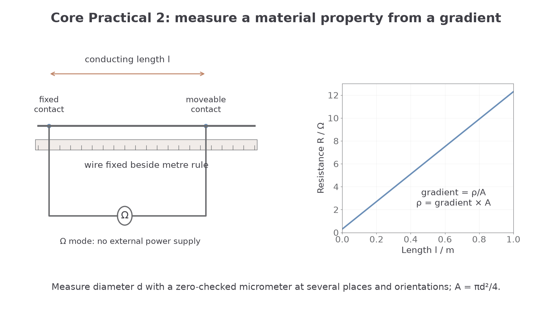
Each piece of apparatus has a job:

the wire is the uniform sample whose resistivity is being found;
the metre ruler gives the conducting length $l$ ;
a crocodile clip fixes one end of the measured length;
a moveable plug or contact touches the wire at different lengths;
a digital multimeter on its lowest ohms range measures the resistance $R$ ;
a micrometer screw gauge measures the small wire diameter accurately.

A clean method is:

Fix the wire straight along a metre ruler and connect one end with a crocodile clip.
Touch the moveable contact to the wire at about $0.10\,\mathrm{m}$ from the fixed end.
Record the length $l$ from the fixed end and the resistance $R$ .
Move the contact along the wire in equal steps, such as $0.10\,\mathrm{m}$ , recording $R$ and $l$ each time.
Measure the wire diameter with a micrometer at several positions and in two perpendicular orientations where possible.
Calculate the mean diameter and then the cross-sectional area.
Plot $R$ on the vertical axis against $l$ on the horizontal axis.
Use the gradient to calculate $\rho$ .

Why graph it instead of using only one length? A graph uses all the readings and makes scatter visible. It also helps separate the length-dependent resistance of the wire from a roughly constant extra resistance caused by contacts or meter leads.

The graph should be straight for a uniform wire at constant temperature. From

R = \rho \frac{l}{A}

compare with

y = mx + c

If $R$ is on the vertical axis and $l$ is on the horizontal axis, the gradient is

m = \frac{\rho}{A}

\rho = mA

The intercept may not be exactly zero. A non-zero intercept can come from contact resistance, meter-lead resistance or a small zero error. A constant positive lead/contact resistance shifts the line upward; a calibration or length-zero offset can shift it either way. The gradient isolates the wire contribution only while these offsets and temperature remain stable.

One practical caution is temperature. Resistivity depends on temperature, so the current through the wire should be small and the wire should not be left connected long enough to heat up. Heating changes the material while you are trying to measure it.

Before taking readings, close the micrometer gently with its ratchet and check its zero. The ratchet applies a consistent force; overtightening can compress a thin wire. Correct a measured zero error and take readings at several locations and perpendicular orientations to test whether the wire is uniform and circular. Read the wire’s actual contact points against the ruler, not the ends of the clip bodies. Avoid stretching the wire, because this alters its area.

An ohmmeter supplies its own small measuring current: use it on a disconnected, unpowered sample. Do not connect an external supply to a meter set to resistance. Check the resistance of the joined leads and use secure contacts. A constant lead/contact resistance shifts the intercept but not the gradient; if contact resistance changes at each length it causes scatter or bias and is not removed automatically.

A valid alternative is a low-voltage supply with a limiting resistor and an ammeter in series with the sample, and a voltmeter across the measured wire length. Take paired $V,I$ readings and calculate $R=V/I$ at each length. Use small currents, switch off between readings, and avoid touching a hot wire. The graph processing is the same as for the ohmmeter method.

Keep the raw diameter, resistance and length readings in a dated table, with units, resolutions, zero corrections and temperature conditions. Record any changes to the contacts rather than deleting awkward points. A spreadsheet can plot the resistance–length data and fit a gradient and intercept; inspect the residual scatter and do not force the line through the origin when the contacts add resistance.

From Gradient to Resistivity

The graph route is a representation shift: the apparatus gives pairs of $R$ and $l$ ; the graph turns those pairs into one gradient; the gradient turns into the material value $\rho$ .

Suppose a student measures the resistance of different lengths of a constantan wire. A best-fit line through the straight trend includes these two points:

Length $l$ / m	Resistance $R$ / Ω
$0.20$	$2.7$
$0.90$	$11.1$

The micrometer gives a mean diameter of $0.230\,\mathrm{mm}$ .

Worked example: using the best-fit gradient

Decision point 1: use points on the best-fit line, not necessarily two raw data points.

\text{gradient}= \frac{\Delta R}{\Delta l}

\text{gradient}= \frac{11.1 - 2.7}{0.90 - 0.20}

\text{gradient}= \frac{8.4}{0.70} = 12.0\,\mathrm{\Omega\,m^{-1}}

Decision point 2: calculate area from diameter in metres.

d = 0.230\,\mathrm{mm} = 2.30 \times 10^{-4}\,\mathrm{m}

r = 1.15 \times 10^{-4}\,\mathrm{m}

A = \pi (1.15 \times 10^{-4})^{2} = 4.15 \times 10^{-8}\,\mathrm{m^{2}}

Decision point 3: connect the gradient back to the original equation.

Since $\text{gradient}= \rho /A$ ,

\rho = \text{gradient} \times A

\rho = 12.0 \times 4.15 \times 10^{-8} = 4.98 \times 10^{-7}\,\mathrm{\Omega\,m}

So the measured resistivity is about

5.0 \times 10^{-7}\,\mathrm{\Omega\,m}

That is a "determine" style result: the value has been obtained through a quantitative method, not by recalling a number. Edexcel-style credit normally depends on showing the gradient route, using SI units for diameter and area, and giving the final unit.

A common wrong route is to use the intercept as the resistance of the wire. The gradient is what tells you how much extra resistance is added for each extra metre of wire. Resistivity is found from that length-dependent change.

Uncertainty and Evaluation

This practical is often limited by small measurements. The length may be measured to the nearest millimetre, but the diameter may be only a few tenths of a millimetre. A tiny absolute uncertainty in diameter can become a large percentage uncertainty in area.

Because

A = \pi \frac{d^{2}}{4}

the percentage uncertainty in area is approximately twice the percentage uncertainty in diameter.

Worked example: combining the main percentage uncertainties

A student obtains

\text{gradient}= 12.0 \pm 0.5\,\mathrm{\Omega\,m^{-1}}

and

d = 0.230 \pm 0.005\,\mathrm{mm}

Decision point 1: compare uncertainties as percentages.

Percentage uncertainty in gradient:

(\frac{0.5}{12.0}) \times 100\% = 4.2\%

Percentage uncertainty in diameter:

(\frac{0.005}{0.230}) \times 100\% = 2.2\%

Decision point 2: area depends on $d^{2}$ , so double the diameter percentage uncertainty.

Percentage uncertainty in area:

2 \times 2.2\% = 4.4\%

Decision point 3: $\rho = \text{gradient} \times A$ , so add the percentage uncertainties.

Percentage uncertainty in $\rho$ :

4.2\% + 4.4\% = 8.6\%

If $\rho = 5.0 \times 10^{-7}\,\mathrm{\Omega\,m}$ , the absolute uncertainty is about

0.086 \times 5.0 \times 10^{-7} = 0.43 \times 10^{-7}\,\mathrm{\Omega\,m}

so a sensible report is

\rho = (5.0 \pm 0.4) \times 10^{-7}\,\mathrm{\Omega\,m}

Method evaluation should use evidence, not a list of generic improvements:

If the line has a non-zero intercept, discuss contact resistance, meter-lead resistance or zero error.
If points are scattered, discuss random variation in contact pressure or reading instability.
If the wire warms up, resistivity may change during the experiment.
If diameter readings vary around the wire, the sample may not be perfectly uniform or circular.
If diameter uncertainty dominates, take several micrometer readings in different places and orientations, check zero error, and calculate a mean.

For Edexcel “evaluate” or “comment on” prompts, a strong answer names the evidence and links it to the effect on $\rho$ . "Use better equipment" is too vague unless you say which measurement it improves and why.

The Charge-Carrier Model

The practical gives a macroscopic property: resistivity. The microscopic explanation uses

Current and charge carriers

I = nqvA

Symbol	Meaning	Unit
$I$	current	ampere, $\mathrm{A}$
$n$	number of charge carriers per unit volume	$\mathrm{m^{-3}}$
$q$	charge on each carrier	coulomb, $\mathrm{C}$
$v$	mean drift velocity of the carriers	$\mathrm{m\,s^{-1}}$
$A$	cross-sectional area	$\mathrm{m^{2}}$

The equation comes from a moving slice of charge. In a time $\Delta t$ , carriers with drift speed $v$ move a distance $v \Delta t$ . The volume containing the carriers that drift across a section is $A v \Delta t$ . If there are $n$ carriers in each cubic metre, the number passing is $n A v \Delta t$ . Each has charge $q$ , so

\Delta Q = nqA v \Delta t

and because $I = \Delta Q / \Delta t$ ,

I = nqvA

The drift velocity is slow. That does not mean the circuit response is slow. Individual electrons in a metal collide frequently and drift gradually, while the electric field change around the circuit is established very quickly.

Worked example: drift speed in a metal wire

A copper wire has diameter $1.0\,\mathrm{mm}$ and carries current $2.0\,\mathrm{A}$ . The number density of mobile electrons is $8.5 \times 10^{28}\,\mathrm{m^{-3}}$ . Use the charge magnitude of an electron as $1.60 \times 10^{-19}\,\mathrm{C}$ . Calculate the mean drift speed.

Decision point 1: use the magnitude of charge for the speed calculation; direction is a separate idea.

Decision point 2: calculate cross-sectional area from the radius.

r = 0.50\,\mathrm{mm} = 5.0 \times 10^{-4}\,\mathrm{m}

A = \pi (5.0 \times 10^{-4})^{2} = 7.85 \times 10^{-7}\,\mathrm{m^{2}}

Decision point 3: rearrange $I = nqvA$ for $v$ .

v = \frac{I}{nqA}

v = \frac{2.0}{(8.5 \times 10^{28})(1.60 \times 10^{-19})(7.85 \times 10^{-7})}

v = 1.9 \times 10^{-4}\,\mathrm{m\,s^{-1}}

That is less than a millimetre per second. A tempting but wrong idea is that electrons must rush round the whole circuit as soon as the switch is closed. The model says the current is large because the number of mobile carriers is enormous, not because each carrier has a large drift speed.

Here $n$ counts mobile carriers, not all electrons in the atoms. Random thermal motion continues in all directions, but the small net drift produces current. For the magnitude form $I=nqvA$ , use $q$ as the positive charge magnitude and $v$ as the drift speed; electron drift is opposite conventional current. When several types of carriers contribute, their contributions to the conventional current must be combined.

Why Resistivities Vary So Much

The two equations now meet.

R = \rho \frac{l}{A}

connects resistance to the material and shape.

I = nqvA

connects current to the carriers moving through the cross-section.

For the same shape and the same potential difference, a material with a smaller current has a larger resistance. Since $\rho = RA/l$ , a larger resistance for the same length and area means a larger resistivity.

The charge-carrier model explains why the current can be very different:

$n$ may be large, as in a metal with many mobile electrons;
$n$ may be very small, as in an insulator with very few mobile charge carriers;
the drift speed $v$ for a given electric field may be small if carriers collide often or are not very mobile;
the charge $q$ is fixed for electrons, but in other conducting materials, such as electrolytes, the mobile carriers may be ions with different charges.

So a low-resistivity material is not "a material where charges feel no resistance". It is a material where, for a given electric field and sample shape, enough mobile charge passes each second to give a large current. A high-resistivity material gives a much smaller current because there are fewer mobile carriers, less mobile carriers, or both.

This also explains why resistivity is temperature dependent. In a metal, higher temperature usually means stronger lattice vibrations and more collisions, so the drift speed for a given electric field is reduced. In a semiconductor, heating can increase the number of mobile carriers, so the effect can be different. The detailed temperature models come in the next lesson, but the idea is the same: carrier number and carrier motion matter.

For Edexcel “explain” questions, do not stop at "there are more charge carriers." Link the chain:

Larger $n$ or $v$ → larger $I$ through the same area → smaller $R$ for the same p.d. → smaller $\rho$ for the same $l$ and $A$ .

or the reverse chain for a high-resistivity material.

Last Accessed

Topic 1: Working as a Physicist

Topic 2: Mechanics

Topic 3: Electric Circuits

Topic 4: Materials

Topic 5: Waves and Particle Nature of Light

Topic 6: Further Mechanics

Topic 7: Electric and Magnetic Fields

Topic 8: Nuclear and Particle Physics

Topic 9: Thermodynamics

Topic 10: Space

Topic 11: Nuclear Radiation

Topic 12: Gravitational Fields

Topic 13: Oscillations

39-41 - Resistivity and Charge Carriers (CP2)