161-163 - Doppler Shift, Hubble’s Law and Cosmology

A Moving Source Changes the Wave Pattern

Picture a fire engine driving past while its siren is on. The siren emits wavefronts at regular time intervals. If the source moves towards you, each new wavefront is emitted from a position slightly closer than the previous one, so the wavefronts arrive closer together: shorter wavelength and higher observed frequency. If the source moves away, the wavefronts are spread out: longer wavelength and lower observed frequency.

That is the Doppler effect. It does not mean the source itself has changed frequency; it means the frequency measured by the observer or detector changes because the source and observer have relative motion along the line joining them.

For light, the same idea appears in spectra. A source moving away has its spectral lines shifted towards longer wavelength. Astronomers call this a redshift because red light is at the longer-wavelength end of the visible spectrum. A source moving towards us would show a blueshift, with spectral lines shifted towards shorter wavelength.

The tempting shortcut is to say "the galaxy looks red". The correct model is sharper: the whole pattern of spectral lines is shifted. The pattern matters because it lets us identify the same element in the laboratory and in the light from a distant galaxy.

From Spectral Lines to Redshift

[DIAGRAM: asset_name: Laboratory lines at 450, 500, 600 nm and observed lines at 486, 540, 648 nm; asset_slug: 047_doppler_redshift_hubbles_law_cosmology__diagram_01; recommended_method: matplotlib; description: Laboratory lines at 450, 500, 600 nm and observed lines at 486, 540, 648 nm; all have redshift 0.080.]

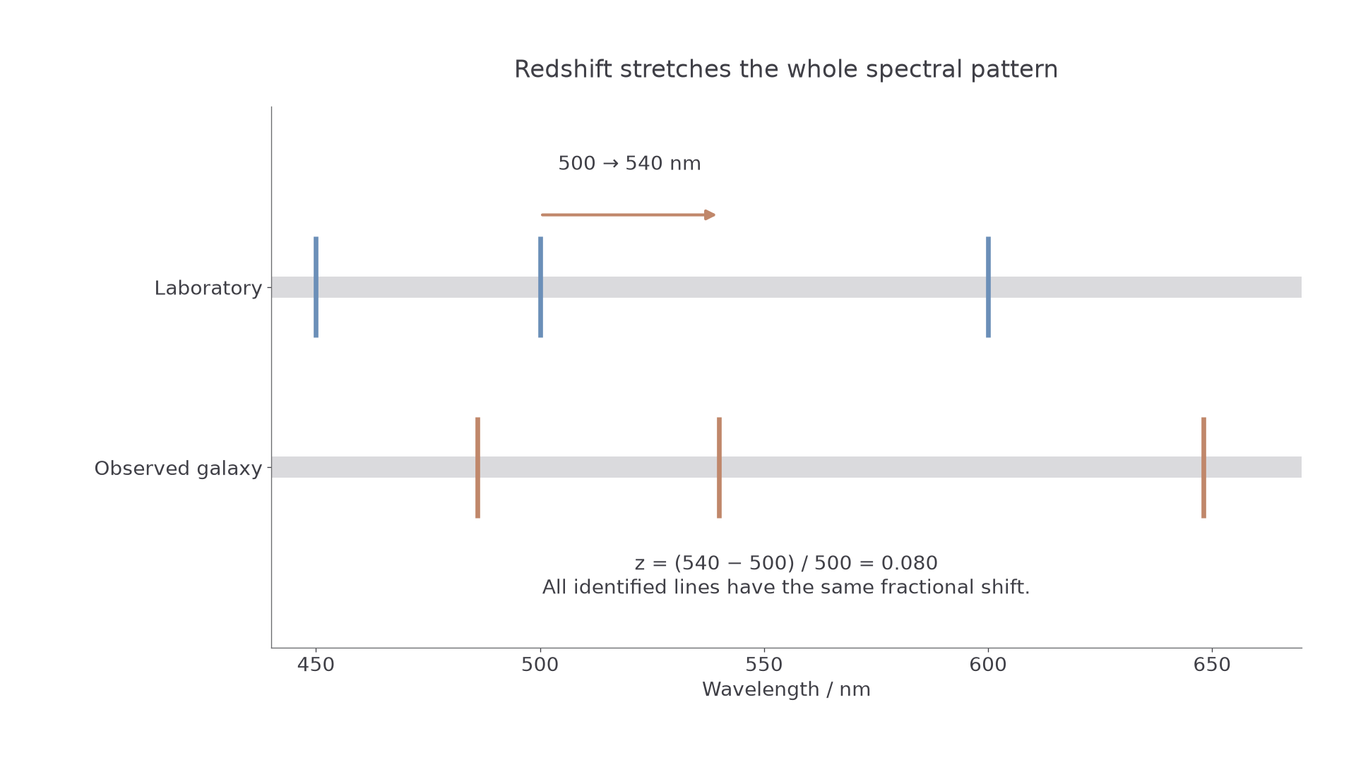
The illustration shows a larger wavelength shift to make the pattern visible. Use the separate numerical readings in each worked example or question.

Redshift is a fractional change:

Here $\lambda$ is the rest wavelength measured in the laboratory and $\Delta \lambda = \lambda_{\mathrm{observed}} - \lambda_{\mathrm{rest}}$. For a redshift, $\lambda_{\mathrm{observed}}$ is larger than $\lambda_{\mathrm{rest}}$, so $\Delta \lambda$ and $z$ are positive.

The Edexcel data/formulae booklet supplies the low-speed relationship:

For frequency, be careful with signs. In a redshift the observed frequency is lower, so $f_{\mathrm{observed}} - f_{\mathrm{rest}}$ would be negative. In this supplied relationship, $\Delta f/f$ is normally used as the size of the frequency decrease when calculating the recession speed.

Worked example: a hydrogen line has a laboratory wavelength of $656.3\,\mathrm{nm}$. In light from a galaxy, the same line is observed at $660.0\,\mathrm{nm}$.

Route: use wavelength because the wavelengths are given. Use $v \approx zc$ only after finding the fractional shift.

Working:

The line has shifted to a longer wavelength, so the galaxy is receding from the observer. In an Edexcel "calculate" item, the credit usually depends on a clear substitution, a final unit for speed, and a sensible number of significant figures.

Hubble's Law as a Graph and an Equation

For objects at cosmological distances, Edexcel supplies Hubble's law:

$v$ is the recession speed in $\mathrm{m\,s^{-1}}$, $d$ is distance in $\mathrm{m}$, and $H_0$ is the Hubble constant. If $v$ is plotted on the vertical axis and $d$ on the horizontal axis, the gradient is $H_0$.

This is a representation shift: the equation says speed is proportional to distance, while the graph says the data should form an approximate straight-line trend through the origin. The gradient is not just a mathematical slope; it is the expansion rate.

Worked example: use the speed from the previous example, $v = 1.69 \times 10^{6}\,\mathrm{m\,s^{-1}}$. A question gives $H_0 = 2.30 \times 10^{-18}\,\mathrm{s^{-1}}$.

Route: rearrange $v = H_0 d$ because distance is unknown. Keep SI units, then convert to megaparsecs if asked.

Working:

Using $1\,\mathrm{Mpc} = 3.09 \times 10^{22}\,\mathrm{m}$,

The unit check is useful: $\mathrm{m\,s^{-1}}/\mathrm{s^{-1}}$ gives metres. A common wrong route is to leave $H_0$ in $\mathrm{km\,s^{-1}\,Mpc^{-1}}$ while using $v$ in $\mathrm{m\,s^{-1}}$; the numerical answer then carries a hidden unit mismatch.