172-173 - Radioactive Decay, Half-Life and Activity

Random nuclei, predictable samples

Imagine a sealed radioactive source beside a detector. The detector clicks when radiation from a decay is detected, but no one can point to one particular unstable nucleus and say, "that one will decay next."

Nuclear decay is spontaneous: it is not caused by ordinary external conditions such as heating, cooling, pressure or illumination. It is also random: for one unstable nucleus, the exact time of decay cannot be predicted.

The useful pattern appears when there are many identical unstable nuclei. Each undecayed nucleus has the same probability of decaying per unit time. That probability per unit time is the decay constant, written $\lambda$.

• $\lambda$ is measured in $\mathrm{s^{-1}}$ if time is measured in seconds.
• A larger $\lambda$ means a greater probability per second, so the source decays faster.
• The nuclei do not take turns or become "due" after waiting for one half-life.

That last point is the key contrast. A half-life is not a timer attached to each nucleus. It is the time for the expected number of undecayed nuclei in a large sample, and therefore the activity, to halve. The individual events remain random; the large-sample trend becomes smooth enough to model.

A sample also does not usually lose half its visible mass or volume after one half-life. What halves is the number of undecayed radioactive nuclei of that isotope. If the sample is mostly stable material with a tiny amount of a radioactive isotope inside it, its visible size may barely change while its activity drops a lot.

Activity is a rate

The activity $A$ of a radioactive source is the number of decays per second. Its unit is the becquerel, $\mathrm{Bq}$, where:

If a sample contains $N$ undecayed radioactive nuclei, and each nucleus has decay probability per unit time $\lambda$, then the expected number of decays per second is:

This equation is more than a substitution rule. It says activity is high when there are many undecayed nuclei left, or when each nucleus has a high probability of decaying each second.

The number $N$ is falling, so its rate of change is negative:

The minus sign is a direction sign: $N$ decreases with time. Activity itself is normally quoted as a positive rate.

Now add the detector. A detector in a lab does not hear only the source; it also records background count rate from natural and environmental radiation. In lesson and exam data, use the corrected count rate when it is standing in for source activity:

In a real experiment, detector efficiency and geometry also matter, but Edexcel questions will state what is needed. The important habit here is not to treat raw count rate as automatically equal to source activity.

Because decay events are random, short counting intervals can fluctuate noticeably. A more reliable activity estimate comes from counting for longer, or repeating counts and taking a mean, then subtracting a background count measured in the same units.

Worked route:

A source contains $3.0 \times 10^{12}$ undecayed nuclei of a radioactive isotope. Its decay constant is $2.0 \times 10^{-6}\,\mathrm{s^{-1}}$. Calculate the activity.

Choose $A = \lambda N$ because the question gives the number of undecayed nuclei and the decay constant.

The unit works because $N$ is a count, so the $\mathrm{s^{-1}}$ from $\lambda$ becomes decays per second. A tempting wrong route is to use half-life immediately, but no half-life is given or needed.

You can model the rate equation in small time steps without solving a differential equation. Over a short interval $\Delta t$, the expected change is $\Delta N\approx-\lambda N\Delta t$, so $N_{\text{next}}=N(1-\lambda\Delta t)$. In a spreadsheet, enter time and N in adjacent columns, increase time by $\Delta t$, and multiply the previous N by this factor in each new row. For $N_0=10000$, $\lambda=0.020\,\mathrm{s^{-1}}$ and $\Delta t=1\,\mathrm s$, the first estimates are 10000, 9800 and 9604. The loss gets smaller as N falls. Choose $\lambda\Delta t\ll1$ and repeat with a smaller step to check convergence; these values are expected populations, not predictions of individual decay events.

Determining half-life graphically

Half-life can be determined from a graph of background-corrected count rate against time, or from a graph of the number of undecayed nuclei against time. Both quantities halve in the same time because $A = \lambda N$.

[DIAGRAM: asset_name: Corrected count rate 80 times 2 to the power minus t/3, against hours; asset_slug: 050_radioactive_decay_half_life_activity__diagram_01; recommended_method: matplotlib; description: Corrected count rate 80 times 2 to the power minus t/3, against hours; halves at 3,6,9 hours; companion natural-log straight line.]

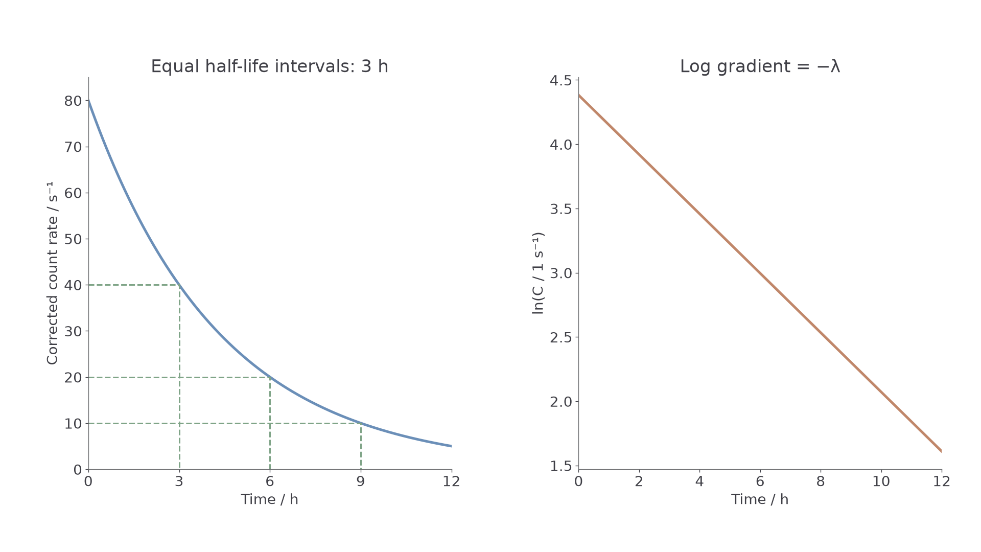
The graph method is:

1. Start from a background-corrected count rate on the curve.
2. Halve that activity.
3. Read horizontally to the curve at the halved activity.
4. Read down to the time axis.
5. The time difference between the two readings is the half-life.