53-57 - Hooke’s Law, Stress and Young Modulus (CP5)

Stiffness as a Graph Gradient

Start with a wire, spring or elastic strip hanging from a clamp. Add a small load and the marker moves. Add another equal load and, while the object is behaving simply, the marker moves by the same extra distance again. The extension is acting like a visible record of the extra force.

Hooke's law for this region is

The $\Delta$ matters. A graph might not begin at exactly zero because there is a small preload, a zero error or an initial hanger. Stiffness is found from a change in force divided by the corresponding change in extension:

$k = \Delta F / \Delta x$

On a force-extension graph with force on the vertical axis and extension on the horizontal axis, the gradient of the straight-line part is $k$.

Worked example: finding stiffness from a straight-line graph

A spring is tested in its straight-line region. When the force increases from $2.0\,\mathrm{N}$ to $8.0\,\mathrm{N}$, the extension increases from $4.0\,\mathrm{mm}$ to $16.0\,\mathrm{mm}$.

Decision point 1: use changes, not just one reading.

$\Delta F = 8.0 - 2.0 = 6.0\,\mathrm{N}$

Decision point 2: convert millimetres to metres before calculating $k$.

If the force then rises by another $3.0\,\mathrm{N}$ while the graph is still straight, the extra extension is

That last sentence hides a condition: only use the same $k$ while the object is still in the proportional region. Once the graph curves, the object no longer has that same constant stiffness.

A common trap is to say "the gradient is extension divided by force" because extension is the thing that changes visibly. That is only true if extension is plotted on the vertical axis. Read the axes first. On the usual force-extension graph, gradient is $\text{force} / \text{extension}$, so it has units $\mathrm{N\,m^{-1}}$.

From Object Stiffness to Material Stiffness

Stiffness $k$ belongs to a particular object. A short thick copper wire is stiffer than a long thin copper wire, even though both are made of copper. To compare materials fairly, we stop asking only "how much force?" and "how much extension?" and instead ask:

• How much force acts on each square metre of cross-section?
• What fraction of the original length has been added or compressed?

Strain has no unit because it is a length divided by a length. It can be written as a decimal or percentage, but the Young modulus equation uses the decimal form. Young modulus is therefore measured in pascal. A larger Young modulus means a material needs a larger stress for the same strain, so the linear part of its stress-strain graph is steeper.

Worked example: turning wire measurements into Young modulus

A wire has original length $2.50\,\mathrm{m}$ and diameter $0.40\,\mathrm{mm}$. A tensile force of $12.0\,\mathrm{N}$ causes an extension of $2.2\,\mathrm{mm}$.

Decision point 1: cross-sectional area uses radius, not diameter.

Decision point 2: stress is force divided by area, not force divided by length.

Decision point 3: strain uses the original length of the wire, not the final length.

Decision point 4: Young modulus has the same unit as stress because strain has no unit.

This is why Young modulus is more powerful than stiffness. If the same material is made longer or thinner, $k$ changes. The value of $E$ should stay approximately the same while the material is in its linear elastic region.

Misconception contrast: "a thicker wire has a larger Young modulus" is not the right model. A thicker wire has a larger stiffness for the same length because its area is larger. Young modulus is the material comparison after area and length have been accounted for.

The same definitions apply to compression: compressive stress is the compressing force divided by cross-sectional area, and compressive strain is the decrease in length divided by original length. For example, a block of area $2.0\times10^{-4}\,\mathrm{m^2}$ shortened by 0.040 mm from 0.10 m under 800 N has stress $4.0\times10^6\,\mathrm{Pa}$, strain $4.0\times10^{-4}$ and, if proportional, $E=1.0\times10^{10}\,\mathrm{Pa}$. Compression and tension can be plotted as positive magnitudes provided the axes say which is used.

Graph Landmarks and Deformation

Force-extension, force-compression and stress-strain graphs tell the same story at different scales. The force-extension graph describes one object. The stress-strain graph describes the material more generally.

[DIAGRAM: asset_name: material graph landmarks; asset_slug: 9ph0_material_landmarks; recommended_method: matplotlib; description: Illustrative tensile stress–strain graph with proportionality/yield/fracture labels and a separate loading–unloading graph showing permanent extension.]

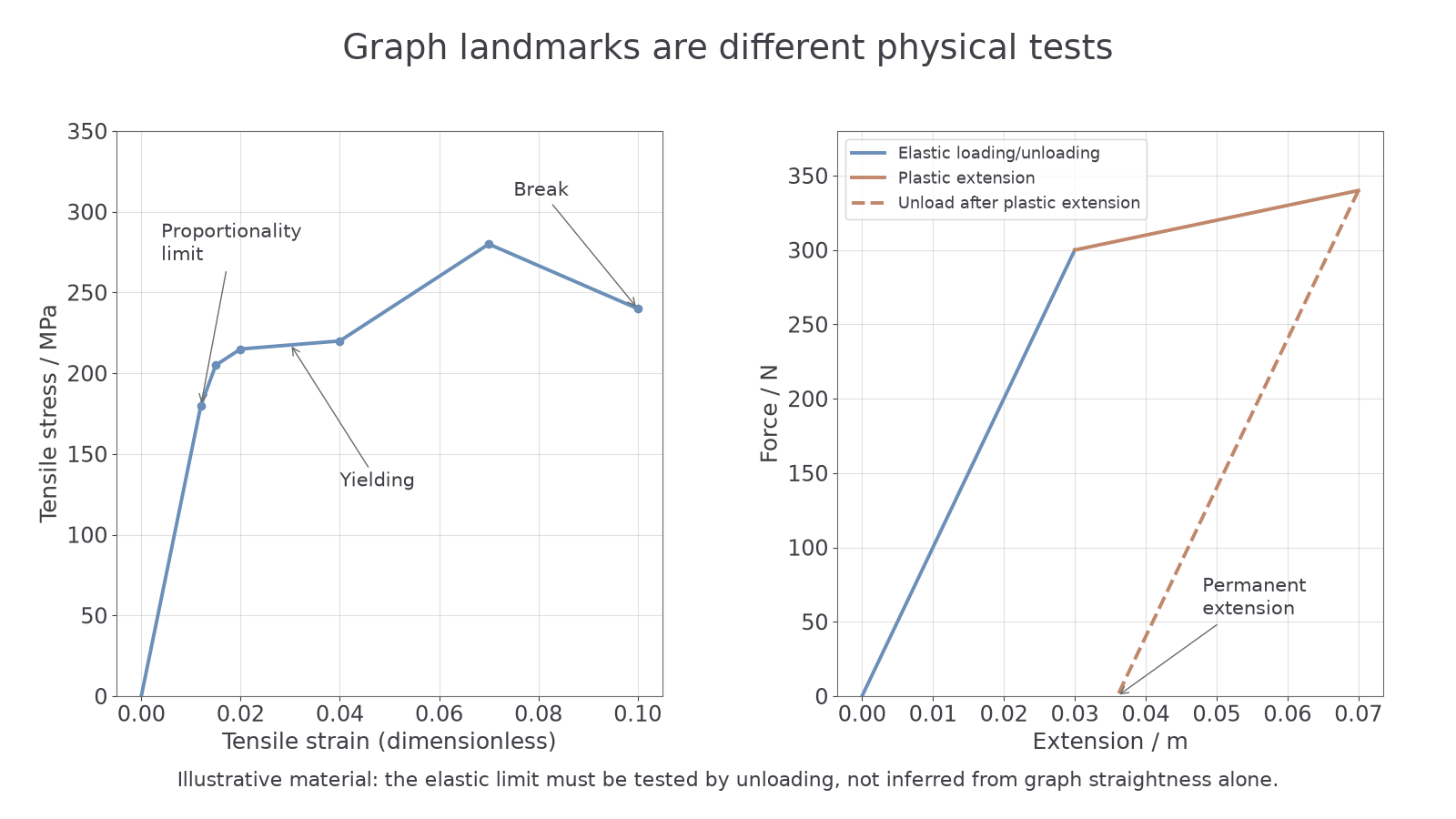
In the first straight section, force is proportional to extension and Hooke's law applies. On a force-extension graph, the gradient is stiffness. On a stress-strain graph, the gradient is Young modulus.

After the limit of proportionality, doubling the force no longer doubles the extension. Beyond the elastic limit, some permanent deformation remains. It is often confused with the limit of proportionality, but the ideas are not the same. The limit of proportionality is about graph straightness and Hooke's law. The yield point is about the onset of yielding/plastic flow.

Breaking stress belongs on a stress-strain graph because it is a stress value, not simply a force value.

For compression, the same ideas apply but the change in length is a compression rather than an extension. Some graphs use positive compression values to keep the graph easy to read. If signs are used, choose a direction and stay consistent.

To sketch these graphs, put force on the vertical axis and extension or compression on the horizontal axis. The proportional region is a straight line through the origin with gradient $k$; mark where it stops being straight and distinguish that point from the recovery-on-unloading elastic limit. For a stress-strain graph, label stress vertically and strain horizontally: the initial gradient is $E$. Show yielding as a large strain increase for little additional stress, and mark the breaking stress as the stress coordinate where the sample fails. After plastic deformation, unloading leaves a non-zero change in length when the force returns to zero.

One boundary matters here: the area under a force-extension graph leads into elastic strain energy, which is the next lesson. In this lesson, use these graphs mainly for gradients, linear regions and deformation landmarks.