9.1.11, 3.2.2, D.1.8, D.1.13, D.2.2 - Spearman’s rank decisions
Learn to rank paired co-variable scores, calculate Spearman’s rho and distinguish a correlation’s direction and strength from its significance and causal meaning.
Choosing Spearman for a ranked association
Spearman’s rank measures whether the ordering of people on one co-variable tends to match or reverse their ordering on another.
Spearman’s rho
A rank-based correlation coefficient, written or , which measures the direction and strength of a monotonic association between two co-variables.
Co-variables are the two measured variables in a correlation. For example, a researcher could measure each volunteer's weekly practice time and number of task errors. There is one pair of scores per person, but the aim is an association, not a difference between two conditions. Calling these an IV and DV would suggest an experimental manipulation that this correlational design does not have.
Spearman needs data that can be ranked: at least ordinal measurement on both co-variables. It can also rank numerical measurements when a normality-based method is inappropriate. Inspect a scatter diagram first. A monotonic relationship tends in one direction as the other variable increases; it need not form a straight line. A U-shaped relationship can be clear in a plot yet have a small rank correlation because the direction reverses. Individual participants should be independent of one another.
The sign gives direction. A positive coefficient means that higher scores on one co-variable tend to accompany higher scores on the other; a negative coefficient means higher scores tend to accompany lower scores. The magnitude, , gives rank-association strength: values nearer 1 are stronger, and values nearer 0 show little monotonic association. Neither sign means “good” or “bad”, and a negative association can be just as strong as a positive one.
Ranking each co-variable and handling ties
Rank the scores separately within each co-variable, but preserve the link between each person's two scores.
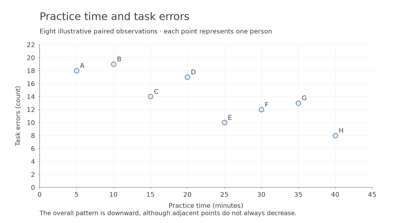
These illustrative data describe eight fictional volunteers' practice time and task-error scores. They demonstrate analysis, not an actual completed investigation. Use ascending ranks for both variables: the lowest practice time receives rank 1, and the lowest error score also receives rank 1. Ranking one variable upwards and the other downwards would reverse the sign artificially.
| Person | Practice time, minutes | Task errors | Practice rank | Error rank | ||
|---|---|---|---|---|---|---|
| A | 5 | 18 | 1 | 7 | −6 | 36 |
| B | 10 | 19 | 2 | 8 | −6 | 36 |
| C | 15 | 14 | 3 | 5 | −2 | 4 |
| D | 20 | 17 | 4 | 6 | −2 | 4 |
| E | 25 | 10 | 5 | 2 | +3 | 9 |
| F | 30 | 12 | 6 | 3 | +3 | 9 |
| G | 35 | 13 | 7 | 4 | +3 | 9 |
| H | 40 | 8 | 8 | 1 | +7 | 49 |
The ranks in each column sum to , and the squared differences sum to 156. The positive and negative differences sum to zero, but their squares do not cancel. Squaring −6 gives +36, not −36.
[DIAGRAM: asset_name: Practice time and task errors; asset_slug: edexcel_9ps0_d07_practice_scatter; recommended_method: deterministic_plot; description: Exact scatter plot of eight illustrative practice-time and task-error pairs with labelled axes and no fitted causal line.; caption: Higher practice times generally accompany fewer task errors, with several local reversals.]
Equal scores need equal ranks
If a co-variable contains ties, assign each tied score the mean of the positions it occupies, then continue with the next unused rank. For a separate five-person illustration, X scores receive ranks . Corresponding Y scores receive ranks . The differences are and . The tie does not reduce N: all five paired observations remain.
Mean ranking correctly handles the ordering, but ties affect the calculation formula. The simple rank-difference formula taught below is exact when neither variable has ties. Applying it to this tied illustration gives .825, while the correlation of the mean-rank columns is about .821. They are close but not identical. Do not label .825 the exact tied-data coefficient. For research with ties, use a properly tie-aware rank-correlation method; in an examination follow the supplied instructions and identify an approximation if that is what is requested. The assessed full calculation in this lesson uses untied data.
Calculating rho from squared rank differences
The supplied formula transforms the total squared rank disagreement into a coefficient between −1 and +1 for untied data.
Continue this lesson.
You’re previewing NovaLearn without an account. Create a free account to read the rest.
Create free account