2.5.1, 2.2.1, 2.2.2, 2.2.3, 2.2.4, 2.2.5, 2.2.6, 2.2.7, 2.2.8, 2.2.9, 2.2.10, 2.2.11, 2.2.12 - Cognitive laboratory investigation
Plan and conduct an ethical laboratory investigation of acoustic similarity and immediate word recall. Apply experimental decisions, present quantitative results, use a suitable non-parametric difference test and write a report. The worked dataset is synthetic: completing this lesson does not establish that you have conducted the required practical.
The memory question and variables
A laboratory experiment manipulates a variable under controlled conditions so that its effect on a measured outcome can be examined.
Our practical asks whether sound similarity affects immediate recall of ten spoken words. The independent variable is list type: acoustically similar or acoustically dissimilar words. The dependent variable is the number of words reproduced in their correct serial positions within 30 seconds immediately after presentation, from zero to ten. This operationalisation makes “memory” measurable and scoring objective. A word recalled in the wrong place is not correct under this rule. Decide spelling rules before testing: a recognisable intended word can count if that rule applies consistently.
A directional experimental hypothesis predicts fewer correct-position words after the similar list than after the dissimilar list. A non-directional hypothesis predicts a difference without stating which condition will be higher. The matching null hypothesis states that there is no difference in correct-position recall in the population; any sample difference is due to chance variation. A directional prediction must be justified in advance, for example by established acoustic-confusion evidence, not chosen after inspecting the scores. The worked analysis below uses the non-directional hypothesis and a two-tailed test at 5%.
Illustrative materials for a pilot are:
| Similar list | Dissimilar list |
|---|---|
| cat, bat, hat, mat, rat, cap, map, tap, lap, gap | dog, sun, pen, cup, fish, tree, book, shoe, bell, road |
Both contain ten one-syllable familiar nouns, but frequency and imagery have not been formally matched. Pilot them and improve problematic items; using multiple matched list sets reduces the risk that an idiosyncratic item drives the result. The similar list contains recurring sounds that can be confused. The task applies an acoustic-memory question without claiming to replicate every feature of Baddeley’s study.
A field experiment could manipulate list type in an ordinary setting, potentially increasing realism but giving less control over noise and interruptions. The specified practical uses a quiet controlled room: a laboratory is defined by the controlled procedure, not necessarily a specialist building. A correlation between age and memory score would answer a different question and would not manipulate acoustic similarity.
Design, sample and control
The design must separate list effects from differences in people and in when they complete each condition.
Use repeated measures, with each consenting participant completing both lists. Pairing scores controls stable participant characteristics such as baseline verbal memory. It creates possible order effects: participants may practise the technique, become tired, or carry material from one list into the next. Counterbalance the order by randomly assigning half to similar-first and half to dissimilar-first, as closely as possible for an odd sample. Include the same short rest interval and different words in the two conditions. Counterbalancing spreads systematic order effects; it does not erase them or prove no carry-over occurs.
An independent-groups alternative avoids participants experiencing both conditions but risks between-person differences; random allocation helps balance these. Matched pairs would pair different participants on a relevant baseline measure before allocating partners to conditions, but matching is time-consuming and cannot equate every characteristic. Do not confuse random assignment to list order with random sampling from a population.
An opportunity sample of adult volunteers available in a college setting is feasible, provided participation is not pressured. It is unlikely to represent all ages, languages or memory abilities. State recruitment criteria, sample size, relevant language/hearing requirements and the limits of the target population. Recruiting more volunteers can improve sensitivity but does not turn an opportunity sample into a representative one. Conduct only an approved, safe investigation with appropriate supervision and accessible consent.
Situational variables include room noise, interruptions and equipment volume; participant variables include fatigue and proficiency in the list language. Standardise instructions, one-word-per-second presentation, recall time, room conditions and scoring. An extraneous variable becomes a confound if it changes systematically with condition: for example, using a quiet room for the dissimilar list and a noisy corridor for the similar list could explain the difference.
Experimenter emphasis or different encouragement can influence results. Use recorded stimuli or a precisely timed script, neutral feedback and, where feasible, a scorer unaware of condition. Demand characteristics arise when participants infer the aim and change their behaviour, such as deliberately rehearsing one list more. Give an honest general description without unnecessarily announcing the exact prediction, and explain the specific aim during debriefing. Do not deceive participants about risks or their right to withdraw.
An ethical and repeatable procedure
The practical needs a procedure another researcher could follow and safeguards that remain active throughout participation.
Provide an accessible information sheet explaining the word-recall task, approximate duration, voluntary participation, possible mild frustration, how data are stored and the withdrawal deadline. Obtain informed consent and use coded identities; keep any contact or consent records separately from scores. Make clear that this is not an intelligence test or clinical assessment, and never display individual rankings publicly. Avoid recruiting people because of a suspected condition or requesting diagnoses. Check hearing and language accessibility without collecting unnecessary sensitive information.
Pilot instructions and materials with volunteers who will not be included in the main dataset. Confirm that words are understandable, the timing is practical and scores avoid being mostly zero or ten. Revise before the main collection and record the change. A pilot is not a way to keep trying changes until a desired significant result appears.
For the main procedure, assign a code and randomised counterbalanced order. Seat the participant in the same quiet setting and give a standard practice example using different words. Present the first ten-word list at one word per second without letting the participant see it. Immediately provide a numbered response sheet and allow 30 seconds to write the words in order. Remove the response sheet, give a standard one-minute rest and repeat for the other condition. Use the predefined scoring rule, record both totals and order, and debrief. Check whether the participant wishes to retain or withdraw their contribution within the agreed arrangements. Permit stopping at any point without pressure.
This procedure allows real collection of paired quantitative data. Save anonymous raw scores, decisions and deviations, such as an interruption, without quietly deleting unfavourable results. Decide exclusion rules before analysis and report them transparently. Anonymised data cannot always be located for later withdrawal; explain that limit honestly in advance. In a report, say what actually happened rather than copying this plan as if it had been performed.
Describing and displaying recall
Descriptive statistics summarise the observed scores before an inferential test considers chance variation.
The following synthetic demonstration data are not a learner’s completed investigation. Each row represents one illustrative participant’s paired scores.
| Code | Dissimilar | Similar |
|---|---|---|
| P1 | 6 | 7 |
| P2 | 6 | 5 |
| P3 | 7 | 5 |
| P4 | 8 | 5 |
| P5 | 9 | 5 |
| P6 | 10 | 5 |
| P7 | 10 | 4 |
| P8 | 10 | 3 |
| P9 | 8 | 8 |
Dissimilar scores sum to 74, so the mean is 74/9 = 8.22 words; similar scores sum to 47, giving 5.22 words. Sorting each list gives medians 8 and 5. The modal scores are 10 and 5; ranges are 10−6 = 4 and 8−3 = 5. For example, five of nine similar scores equal five, or 5/9 × 100 = 55.6%. A frequency table records the count for each score: for the similar list, 3:1, 4:1, 5:5, 6:0, 7:1 and 8:1. Include zero-frequency categories when needed to retain the scale.
Sample standard deviation: .
For the dissimilar list, the sum of squared deviations is 21.5556 and the denominator is 8, so s = 1.64 words to two decimal places. For the similar list, the corresponding sum is 17.5556 and s = 1.48 words. Range depends only on extremes; SD uses all deviations from the mean. Here the similar condition has a larger range but a smaller SD because most scores cluster at five. Neither statistic alone shows significance.
[DIAGRAM: asset_name: Demonstration recall means; asset_slug: edexcel_9ps0_c09_practical_recall_means; recommended_method: deterministic_plot; description: Exact means from the nine synthetic paired scores, 8.22 for dissimilar and 5.22 for similar, on a zero-to-ten correct-position recall axis.; caption: Synthetic condition means describe the sample difference but do not themselves establish significance.]
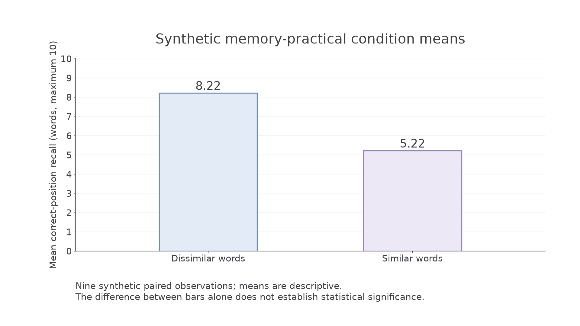
A bar chart is suitable for comparing the two discrete list conditions: labelled category axis, mean number correct on the vertical axis, common zero baseline and separate bars. For a score-frequency display, show scores and their frequencies. A histogram is appropriate for a quantitative distribution grouped into contiguous intervals, with adjacent bars and, for unequal intervals, frequency density so area represents frequency. A frequency polygon joins frequencies at class midpoints. Do not draw a continuous line between list categories as if the conditions were time points.
In your notebook, construct the condition-mean bar chart from the raw table and check labels, scale and heights against the supplied figure; this construction is ungraded here. Normal distributions are approximately symmetric, with similar mean, median and mode. A tail towards high scores indicates positive skew; a tail towards low scores indicates negative skew. A small, bounded recall sample with ceiling scores need not be normal. Inspect the raw distribution rather than declaring it normal because a mean can be calculated.
Testing the paired difference
Wilcoxon signed ranks is suitable here because the question concerns a difference between paired conditions using scores that can be meaningfully ordered.
For independent groups with ordinal or suitably ranked scores, use Mann–Whitney U instead. Its ranks are pooled across the two groups and its observed statistic is the smaller U; it is not the paired-difference procedure below. Choose design, test, tail and significance level before examining the result. The full general methods are taught in the shared skills lessons; here they are applied to the cognitive practical.
Subtract similar from dissimilar consistently. Exclude zero differences from ranking and from N; rank absolute nonzero differences from smallest to largest, using mean ranks for ties. Then restore the signs to identify the two rank totals.
| Code | Dissimilar−similar | Absolute difference | Rank | Sign |
|---|---|---|---|---|
| P1 | −1 | 1 | 1.5 | Negative |
| P2 | +1 | 1 | 1.5 | Positive |
| P3 | +2 | 2 | 3 | Positive |
| P4 | +3 | 3 | 4 | Positive |
| P5 | +4 | 4 | 5 | Positive |
| P6 | +5 | 5 | 6 | Positive |
| P7 | +6 | 6 | 7 | Positive |
| P8 | +7 | 7 | 8 | Positive |
| P9 | 0 | 0 | Excluded | Excluded |
The equal absolute differences of one occupy positions 1 and 2, so both receive (1+2)/2 = 1.5. Positive ranks total 34.5; negative ranks have total magnitude 1.5. Therefore T = 1.5, the smaller total, and N = 8, not nine. Rank totals add to 36, equal to 8×9/2, a useful check.
| Current Pearson Wilcoxon table: N | One-tailed 0.05 / two-tailed 0.10 | One-tailed 0.025 / two-tailed 0.05 | One-tailed 0.01 / two-tailed 0.02 |
|---|---|---|---|
| 8 | 5 | 3 | 1 |
The two-tailed 5% column gives critical T = 3. For Wilcoxon, significance requires observed T equal to or less than critical T. Since 1.5 ≤ 3, reject the null at the chosen level using the supplied Pearson table. The medians and raw scores indicate lower recall for the similar list. A small T indicates most ranked differences favour one condition; “larger statistic = more significant” would be wrong here. Mann–Whitney also uses U ≤ critical under Pearson’s smaller-U convention.
Significance levels of 10%, 5% and 1% set increasingly strict thresholds for rejecting a true null. At 5%, the test procedure limits the long-run probability of a Type I error, rejecting a true null, under its assumptions. It is not a 95% probability that the hypothesis is true. A stricter threshold generally reduces Type I risk but can increase Type II error, failing to reject a false null. Small samples and noisy measurement can also reduce sensitivity. The result does not prove no confounds, a large practical effect, or that every participant showed the predicted pattern. P1 goes the other way and P9 shows no difference. Use the current 2026-onward Pearson formulae and tables and read both tail headers; do not choose a column by its position in an older table.
Reporting and improving the investigation
A scientific report separates the procedure, observed results and interpretation so another reader can judge the conclusion.
In Procedure, state actual recruitment, consent, design, materials, allocation to order, presentation rate, response timing, scoring, debriefing and any deviations. In Results, give anonymous raw data or a clearly labelled table, descriptive statistics, an appropriate graph, test choice, observed statistic, N or sample sizes, tail, alpha, critical value and decision. In Discussion, answer the hypothesis, connect cautiously to acoustic confusion, examine competing explanations and suggest justified improvements. Do not describe synthetic figures as data you collected.
Objectivity is improved by a predefined scoring rule and a scorer unaware of condition. Reliability can be checked by agreement between scorers on the same responses, or replication using equivalent materials; simply repeating the same list risks practice. Internal validity concerns whether similarity caused the difference rather than list familiarity, order or environmental differences. Ecological validity concerns relevance to everyday memory; isolated words with rapid serial recall may not represent meaningful conversations. Predictive validity would require evidence that this measure predicts a specified later outcome, such as performance on another verbal task; it cannot be assumed from high scorer agreement.
An improvement must target the actual weakness: matched and piloted word frequencies reduce material confounds; counterbalancing reduces systematic order bias; recorded presentation reduces inconsistent delivery; multiple equivalent lists test whether one set drove the finding. A broader sample may extend generalisability, but changing age or language also requires valid accessible materials. More control can improve internal validity while making the task less natural, so explain that trade-off rather than claiming every improvement increases every form of validity.
For your own practical, retain the real anonymised raw record and write these sections using what occurred, including nonsignificant findings and limitations. A written planning or analysis score assesses understanding; it does not certify practical performance or graph construction.