9.1.10, 2.2.11, 3.2.1, D.1.3, D.1.7, D.3.1, D.3.2 - Tables, charts and correlations
Learn to turn raw observations into frequency tables, bar charts, histograms and scatter diagrams, and to interpret each display accurately. The descriptive-statistics and mathematical codes cover constructing and translating displays; the biological-method code adds co-variables, correlation patterns and limits on causal conclusions.
From raw data to frequency tables
A frequency table counts how often each score or category occurs without losing track of the total number of observations.
Suppose ten participants produce these invented recall scores: 2, 3, 3, 4, 4, 4, 5, 5, 6, 8 words. List the possible observed scores in order, tally each occurrence and record the count as its frequency. Repeated values are separate observations, not duplicates to delete.
| Recall score (words) | Frequency | (words) |
|---|---|---|
| 2 | 1 | 2 |
| 3 | 2 | 6 |
| 4 | 3 | 12 |
| 5 | 2 | 10 |
| 6 | 1 | 6 |
| 8 | 1 | 8 |
| Total | 10 | 44 |
The frequencies sum to ten, matching the raw record. The score with the largest frequency is 4, so the mode is 4 words. To recover the total number of words recalled, multiply each score by its frequency and sum those products. Dividing 44 by ten gives mean recall of 4.4 words. This translates a numerical list into a table and then into an algebraic calculation:
This gives the exact mean when the table lists exact individual score values. For grouped continuous intervals, using midpoints would give an estimate rather than recovering the original exact scores.
For categories such as chosen revision method, count category frequencies without multiplying arbitrary category codes. Frequencies may be converted into percentages using the correct total. Preserve what is counted: responses, observed behaviours and participants are not interchangeable denominators. Use a clear title and column headings with units so another reader can reconstruct what the table means.
Constructing bar charts
A bar chart compares separate categories or conditions, with bar height representing a clearly specified count, percentage or summary value.
In an invented twelve-person survey, six choose flashcards, four choose practice questions and two choose rereading. Place those categories on the horizontal axis and frequency on the vertical axis. Use equal bar widths, clear gaps between categories, and a uniform numerical scale. Start a frequency bar axis at zero so bar height remains proportional to frequency; cutting it off can exaggerate a modest difference.
[DIAGRAM: asset_name: Revision preference frequencies; asset_slug: edexcel_9ps0_d03_categorical_bars; description: Separate category bars with frequencies 6 for flashcards, 4 for practice questions and 2 for rereading on a zero-based uniform frequency axis; caption: A bar chart compares separate revision-method categories.]
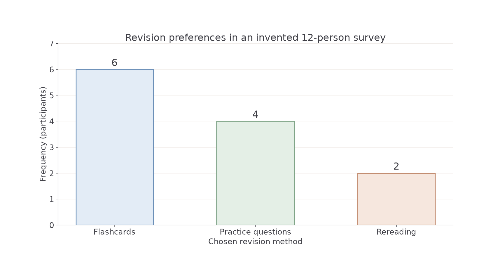
To construct this chart in your notebook, first draw and label both axes. Choose a vertical scale that comfortably includes six, such as one square per participant. Mark 0, 1, 2 and successive equal steps; place equal-width bars reaching 6, 4 and 2. Label the categories and give a title explaining what was measured. Check the chart back against the table rather than drawing bars by eye. Colour can distinguish categories but should not carry information that labels omit.
A bar chart can also compare mean recall under silence and music. Its vertical axis must then say mean recall in words, not frequency. A bar of height 8 would represent an average of 8 words, not eight participants. Include the measurement and relevant condition labels; unequal participant numbers do not justify wider bars. A chart of group means also hides individual variation unless spread is separately supplied.
Ungraded notebook construction: draw the preference chart yourself from the three counts above before comparing it with the supplied image. Check bar heights, equal widths and gaps, zero baseline, units and title. Written Testing can assess your choice and interpretation of a display; it cannot establish that you drew it accurately.
Constructing histograms
A histogram shows how continuous numerical observations are distributed across intervals, with touching bars representing adjacent parts of one scale.
These twelve invented response times, in seconds, are 0.22, 0.24, 0.27, 0.31, 0.32, 0.34, 0.36, 0.37, 0.41, 0.43, 0.46, 0.52. Choose non-overlapping intervals that include every value exactly once:
Continue this lesson.
You’re previewing NovaLearn without an account. Create a free account to read the rest.
Create free account