3.25P-3.27P - Sound speed and oscilloscope practicals

Speed of sound in air

The speed of a wave is the distance travelled by the wave divided by the time taken. For a sound wave travelling through air:

The main practical difficulty is that sound is fast. At room temperature, a sensible result is usually close to 340 m/s, so a short classroom distance gives a very short time. If the distance is too small, human reaction time becomes a large fraction of the reading.

A simple method uses a long measured distance outdoors. One student stands a known distance away and makes a sharp sound, such as clapping two boards together. A second student starts timing when they see the clap and stops timing when they hear the sound. The time taken for the light to reach the observer is negligible at this level, so the measured time is treated as the time taken by the sound.

Another method uses an echo. A student stands a measured distance $d$ from a large flat wall and makes a sharp sound, then times how long the echo takes to return. The sound travels to the wall and back again, so the distance it travels is $2d$, not $d$. The speed is $2d$ divided by the time between the sound and its echo. Using $d$ instead of $2d$ is a common mistake that halves the answer.

To improve the investigation, use a larger distance, repeat the measurement several times, calculate a mean time, and keep background noise low. The calculated speed should be given in m/s because distance is in metres and time is in seconds.

Electronic timing method

An electronic timing method reduces the reaction-time problem. Place two microphones a measured distance apart in a straight line from a sound source. A sharp pulse reaches microphone 1 first and microphone 2 later. The oscilloscope can display the two electrical signals so the time delay between their arrivals can be measured.

[DIAGRAM: asset_name: Sound speed and oscilloscope practicals - diagram 01; asset_slug: p32_sound_speed_and_oscilloscope_practicals__diagram_01; recommended_method: image_gen; description: NovaLearn pale-palette sound-speed practical with sharp source, two microphones separated by measured distance d, unbroken leads to CH1 and CH2, dual pulses with later CH2 onset, matching dashed guides and an on-screen time-delay Δt bracket.]

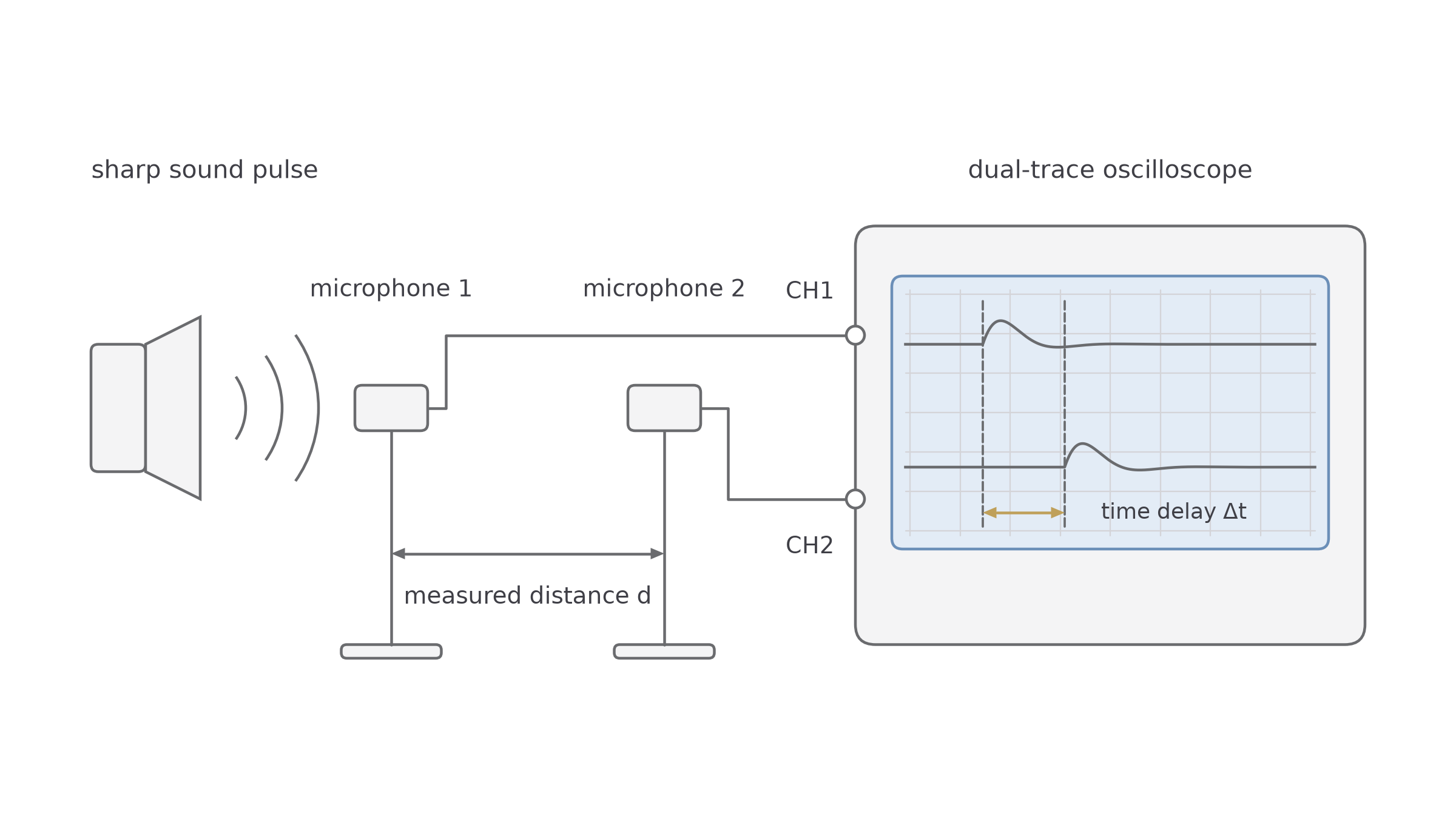
For example, microphones separated by 0.85 m receive the same pulse 2.5 ms apart. Convert first: $2.5\,\mathrm{ms}=0.0025\,\mathrm{s}$. Then $v=0.85/0.0025=340\,\mathrm{m/s}$. Using the source-to-first-microphone distance would not match this measured delay.

For this method:

The distance is not the distance from the sound source to a microphone. It is the extra distance the sound travels between microphone 1 and microphone 2. The time is the delay between the two received signals, not the whole time for the sound to leave the source.

This method still needs careful technique. Place the source outside the interval between the microphones, so the sound reaches them in order along the same line. The microphones should be aligned with the sound source, the room should be quiet, the pulse should be sharp, and the distance between microphones should be measured accurately. Repeating the pulse and using a mean value helps because individual traces can be affected by noise and triggering.

Microphone and oscilloscope

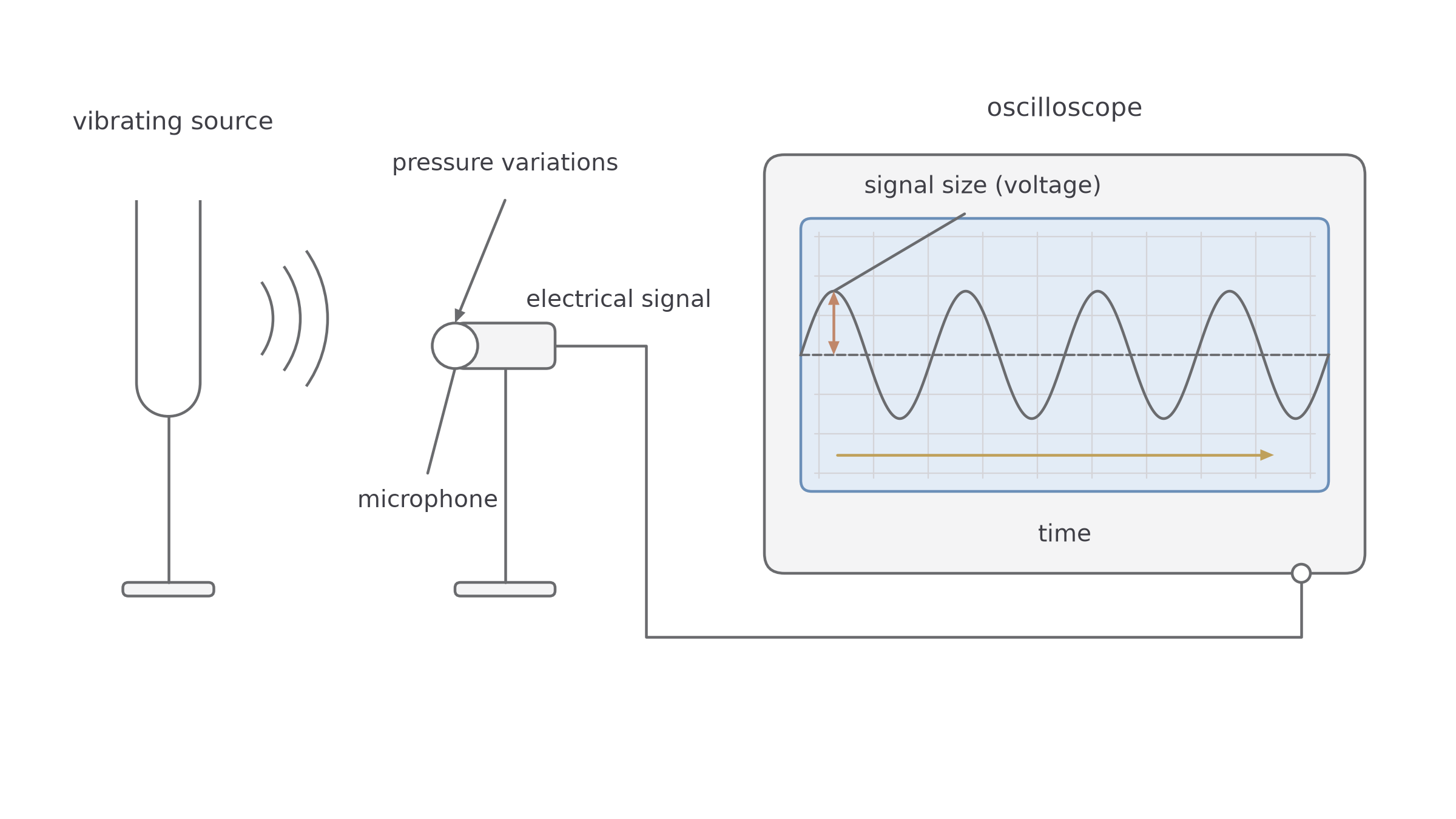
A microphone changes pressure variations in a sound wave into a changing electrical signal. When the microphone is connected to the input of an oscilloscope, the oscilloscope displays that changing signal as a trace.

[DIAGRAM: asset_name: Sound speed and oscilloscope practicals - diagram 02; asset_slug: p32_sound_speed_and_oscilloscope_practicals__diagram_02; recommended_method: image_gen; description: NovaLearn pale-palette vibrating source, microphone head labelled pressure variations to electrical signal, lead to the oscilloscope case, four-cycle trace on a graticule with centreline, rest-to-peak signal-size arrow and time direction.]