Biology 3.12 - 3.14, 3.16 - Inheritance and probability
Explain inherited differences using alleles, then follow one gene through gametes, fertilisation and offspring. Use Punnett squares and family pedigrees to predict and analyse dominant and recessive traits with probabilities, ratios and percentages.
From chromosomes to inherited characteristics
Inherited characteristics pass from parents to offspring in genetic information. In most body cells, chromosomes occur in pairs, with one chromosome of each pair inherited from each parent. A chromosome is a long DNA molecule carrying many genes, and a gene is a section of DNA that codes for a specific protein.
The same gene can occur in different forms called alleles. For a gene considered in a simple inheritance model, an offspring receives one allele from each parent. Different allele combinations can therefore produce differences in an inherited characteristic. Alleles have different DNA base sequences. These can lead to different versions or amounts of a protein, changing how a cell works. For example, one allele may supply a working enzyme that makes a flower pigment, while another supplies an enzyme that does not work. In the simple dominant–recessive model, one working allele may make enough pigment for a coloured flower; two non-working alleles give no pigment. This explains how an inherited DNA difference can cause a phenotypic difference without suggesting that every characteristic follows this one-gene pattern.
| Term | Meaning in a single-gene inheritance model | Example using A and a |
|---|---|---|
| allele | one version of a gene | A or a |
| dominant | an allele expressed in the phenotype when one or two copies are present | A is shown in AA and Aa |
| recessive | an allele expressed in the phenotype only when no dominant allele is present | a is shown in aa |
| homozygous | having two identical alleles for the gene | AA or aa |
| heterozygous | having two different alleles for the gene | Aa |
| genotype | the combination of alleles an organism has for the gene | AA, Aa or aa |
| phenotype | the characteristic shown by the organism | the dominant or recessive form of the characteristic |
| gamete | a reproductive cell carrying one allele for the gene | an egg or sperm carrying A or a |
| zygote | the first cell formed when two gametes fuse at fertilisation | a cell with a two-allele genotype such as Aa |
Dominant and recessive describe the relationship between two alleles. A dominant allele is not necessarily more common, stronger or better, and a recessive allele is not weaker. The capital and lowercase letters are simply symbols used to keep track of which phenotype appears in a heterozygote.
The mechanism can be followed in order:
- A parent has two alleles for the gene in its body cells.
- Each gamete receives one of those alleles.
- At fertilisation, two gametes, one from each parent, fuse.
- The resulting zygote has two alleles, one from each parent.
- That genotype determines the phenotype in the simplified single-gene model.
Building monohybrid crosses
A monohybrid cross follows the inheritance of one gene controlling one characteristic. A genetic diagram shows the parents, the alleles in their gametes and the possible offspring genotypes. A Punnett square organises the same information so that no possible fertilisation is missed.
Use one letter for both alleles. The dominant allele is written as the capital form and the recessive allele as the lowercase form. For example, in a fictional plant, let P be the allele for purple flowers and p the allele for white flowers, with purple dominant.
To construct a cross:
- translate each parent's description into a genotype;
- state the possible one-allele gametes from each parent;
- place one parent's gametes across the top and the other's down the side;
- combine one row allele and one column allele in every box;
- translate each possible offspring genotype into a phenotype.
Worked example: two heterozygous purple plants
Parent phenotypes: purple x purple
Parent genotypes:
Gametes from each parent: P or p
| Parent 2 down / Parent 1 across | P | p |
|---|---|---|
P | PP | Pp |
p | Pp | pp |
The four boxes are four equally likely fertilisation outcomes:
- genotype probabilities: , , ;
- genotype ratio: ;
- purple phenotype:
PPorPp, so ; - white phenotype:
pp, so ; - phenotype ratio: .
As a sense-check, the genotype probabilities add to . The square represents possible zygotes, not four actual offspring that a pair of parents must produce.
Probabilities describe expected outcomes
A Punnett square lets us count equally likely outcomes. Probability, ratio and percentage are different ways to communicate those counts.
Inheritance outcomes
For a ratio, write the number in each requested category in the stated order and simplify if possible.
Worked example: heterozygous x homozygous recessive
In a fictional beetle, smooth wing cases are controlled by dominant allele S; ridged wing cases are controlled by recessive allele s. Cross a heterozygous smooth beetle with a ridged beetle.
Parent genotypes:
Gametes: the Ss parent makes S or s gametes; the ss parent makes only s gametes.
ss parent down / Ss parent across | S | s |
|---|---|---|
s | Ss | ss |
s | Ss | ss |
Two of four boxes show Ss, so the probability of a smooth offspring is
.
Two of four boxes show ss, so the probability of a ridged offspring is also . The genotype ratio is , and the phenotype ratio is .
If this cross produced 80 offspring, the predicted number with ridged wing cases would be
.
For a fixed cross, the probability stays the same, so , where is the total number of offspring. Expected number is therefore directly proportional to the total: doubling the total doubles the expected number with that phenotype.
This is a prediction, not a guarantee. Each fertilisation is a new random event: a probability does not mean smooth and ridged offspring must alternate.
Analysing observed outcomes
Return to the plant cross, which predicts white offspring. Suppose 18 of 80 observed offspring are white:
.
The observed value, , is close to but not exactly the predicted . Chance variation can make a finite set of offspring differ from the theoretical ratio, so a small difference does not by itself show that the genetic model is wrong.
Reading family pedigrees
A family pedigree is a genetic diagram showing relationships and the presence or absence of a tracked phenotype across generations. Its symbols record observations about phenotype; they do not automatically reveal every person's genotype.
The standard key used here is:
| Symbol or line | Meaning |
|---|---|
| square | male |
| circle | female |
| shaded symbol | person shows the tracked phenotype |
| unshaded symbol | person does not show the tracked phenotype |
| horizontal line between two people | parents |
| vertical line to a horizontal sibling line | their children |
Roman numeral and number, such as II-2 | generation and individual identifier |
[DIAGRAM: asset_name: Biology 3.12-3.16 - Inheritance diagrams and probabilities - diagram 01; asset_slug: biology_3_12_3_16_inheritance_diagrams_and_probabilities_diagram_01; recommended_method: image_gen; description: Two-generation fictional family pedigree for a recessive trait where generation I has unaffected male I-1 and unaffected female I-2 joined as parents, and their three generation-II children are unaffected female II-1, affected male II-2 and unaffected male II-3; square means male, circle means female, filled means shows the trait and unfilled means does not show the trait; clear partner, descent and sibling lines; no genotype labels, probability values or medical condition names.]
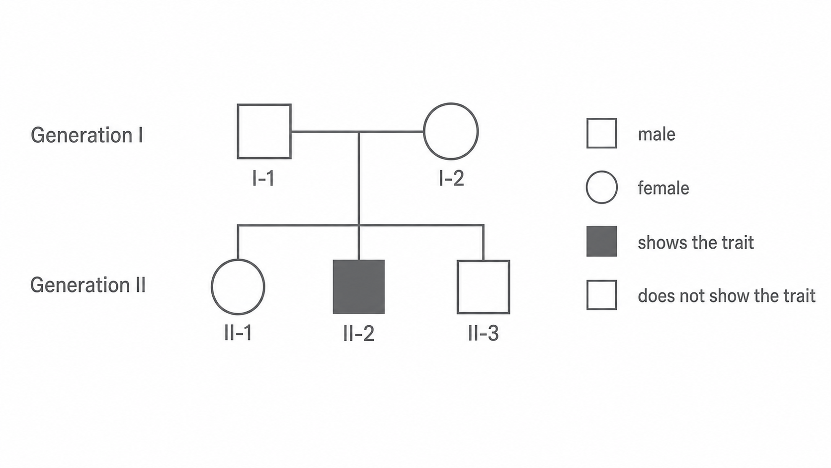
Start pedigree analysis with genotypes that the phenotype forces:
- for a recessive tracked phenotype, a shaded person must be
rr; an unshaded person could beRRorRr; - for a dominant tracked phenotype, an unshaded person must be
dd; a shaded person could beDDorDd.
Then use parent-to-child inheritance: every child receives one allele from each parent.
Worked pedigree inference: a recessive trait
In the diagram, unaffected parents I-1 and I-2 have an affected child, II-2. Let R be the dominant allele and r the recessive allele.
- Because
II-2shows the recessive phenotype, the child's genotype isrr. - The child received one
rfrom each parent, so both parents carryr. - Both parents are unshaded, so neither can be
rr; each must also haveR. - Therefore both parent genotypes are
Rr. - The cross gives , so the probability that any future child shows the trait is .
The unshaded siblings are not automatically RR: each could be RR or Rr. This is why shading alone cannot identify every genotype.
Worked pedigree inference: a dominant trait
Now imagine a different pedigree in which two people show a dominant trait but have a child who does not. Let D be the dominant allele and d the recessive allele.
- The unshaded child must be
ddbecause the dominant phenotype is absent. - The child received one
dfrom each parent, so each parent carriesd. - Each parent shows the dominant phenotype, so each also carries
D. - Both parents must therefore be
Dd. - The cross predicts showing the dominant phenotype and not showing it for each future child.