Biology 1.3 - 1.5 - Microscopy and cell scale
Find out how improved resolution reveals cell structures, estimate sizes and convert between cell-scale units. The final part teaches Higher-tier standard-form calculations.
From larger images to better evidence
A cheek cell is too small to inspect with the unaided eye. A microscope forms a larger
image, but the scientific value of that image depends on whether nearby details can be seen
as separate rather than merging into a blur.
Magnification
Magnification is how many times larger an image is than the object that produced it.
Resolution
Resolution is the ability to distinguish two close points as separate. Higher resolution
reveals finer detail.
These quantities are not interchangeable. Enlarging a low-resolution image makes the blur
bigger; it does not recover missing detail. Useful microscope development has therefore
increased resolution as well as magnification.
A compound light microscope sends visible light through a thin specimen. Objective and
eyepiece lenses form a magnified image. Improvements in lens manufacture, illumination,
staining and image recording have made light-microscope images clearer and easier to compare
than early images.
An electron microscope uses a beam of electrons rather than visible light. Electrons
have a much shorter wavelength than visible light, so electron microscopes can resolve
points that are much closer together. This gives clearer images of organelles and finer
sub-cellular detail. Electron micrographs are usually produced in greyscale; added colour
can help interpretation, but it is not the specimen's natural colour.
The evidence chain is:
improved technology → higher resolution → finer structures distinguished → better
structural evidence → better-supported ideas about function
For example, clearer images reveal the folded inner membrane of mitochondria and allow
scientists to compare the number and position of mitochondria in different cells. Those
observations, combined with experimental evidence about respiration, strengthen the
explanation of a mitochondrion's role. An image alone does not prove a function: it provides
structural evidence that must be connected to other observations and experiments.
Cell scale and estimation
Size is a measurement; scale compares sizes. A bacterium might be about long while an animal cell is about across. The animal cell's measured length is ten times greater, not ten times its volume. These are illustrative estimates: cells vary in size and shape.
A unit prefix tells us the factor relative to one metre.
| Prefix | Symbol | Factor of a metre | One unit in metres |
|---|---|---|---|
| milli | m | ||
| micro | µ | ||
| nano | n | ||
| pico | p |
Each neighbouring step differs by a factor of 1000:
To use a smaller unit, multiply: , because . To use a larger unit, divide: . The object stays the same size; a smaller unit needs a larger number.
When to estimate
An estimate is a reasoned approximate value. Use one when boundaries are unclear, cells vary naturally, a scale can only be read approximately, or a quick check of an answer's size is needed. Give the evidence and unit; an estimate is not an unsupported guess.
For roughly equal cells lying across a known microscope field diameter:
Estimated cell size
If a field spans about 12 cells, the estimated width is . Check: 12 widths of span . Count partial edge cells sensibly and repeat across several fields because cells need not all have the same width.
Higher magnification shows a smaller field on the same microscope. Changing from to multiplies magnification by ten, so a field becomes , or . Use the field diameter for the objective actually in use.
Choosing a graph for cell data
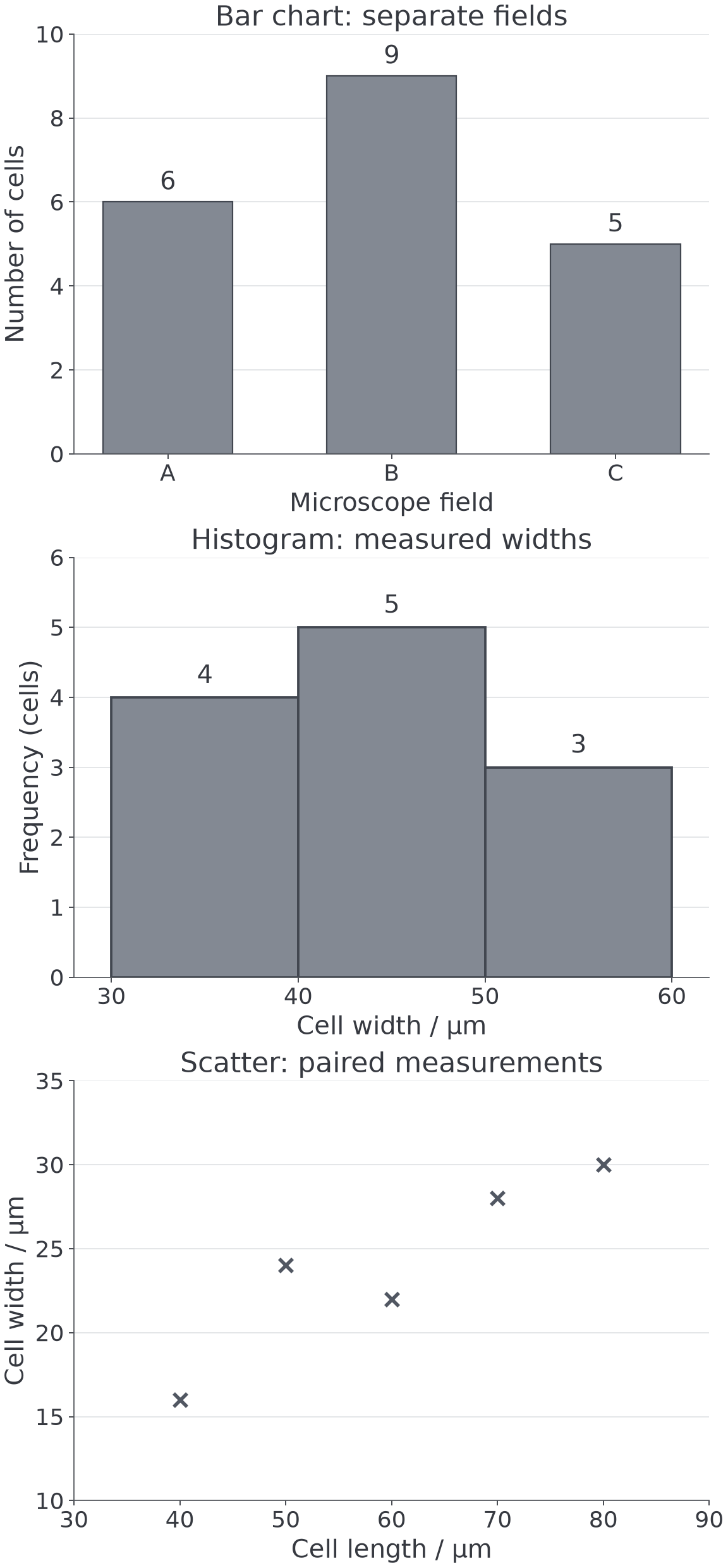
A frequency is how often a value or category occurs. Suppose 12 cells have measured widths of . Count each once into a frequency table:
| Width interval / | Frequency (cells) |
|---|---|
| 4 | |
| 5 | |
| 3 | |
| Total | 12 |
The inequalities prevent double counting: a width of exactly belongs in the second interval. Draw a histogram for this continuous measurement: put width on the horizontal axis and frequency on the vertical axis, and make neighbouring bars touch. All intervals here have equal width, so heights 4, 5 and 3 represent their frequencies. The most frequent interval is ; the grouped graph does not reveal each cell's exact width. With unequal intervals, bar area, not height alone, must represent frequency; use height = frequency ÷ interval width, called frequency density.
Use a bar chart for separate categories. For example, 6, 9 and 5 cells recorded in microscope fields A, B and C give three equal-width bars with gaps. Label the horizontal axis with field names and the vertical axis “Number of cells”, starting at zero. Field B contains three more recorded cells than field A. Do not join category bars into a histogram.
To compare two measurements of the same cells, use a scatter diagram. For five cells, length–width pairs in micrometres are , , , and . Label length on the horizontal axis and width on the vertical axis, choose regular scales covering the data, and plot one point for each pair. Do not connect points in recording order.
The points generally rise to the right: a positive correlation means longer cells tend to be wider, although not every pair follows the trend. A downward trend is negative correlation; no clear trend means no apparent correlation. A sensible best-fit line follows the overall pattern rather than every point. Correlation alone does not show that increasing length causes width to increase.
[DIAGRAM: asset_name: Biology Topic 1 - Graphs of cell data; asset_slug: combined_bio_a_cell_data_graphs; description: Three vertically stacked exact-data plots: category bar chart of fields A/B/C with counts6/9/5 and separated bars; equal-interval histogram of cell widths30–40/40–50/50–60 micrometres with frequencies4/5/3 and touching bars; scatter of length–width pairs(40,16),(50,24),(60,22),(70,28),(80,30) micrometres with an overall positive trend. Clearly labelled axes and units; illustrative data.]
Standard-form calculations
Higher tier only — Biology 1.5(e)
Calculations in this part are Higher content. Knowing the unit prefixes and using ordinary-number conversions in the earlier part remain common to both tiers.
Standard form writes a positive number as , where and is an integer. It keeps very large or very small measurements manageable. For example, .
Worked example
A micrograph image is long. The actual structure is long. Magnification is image size divided by actual size, using the same unit:
- Convert the actual length: .
- Divide image size by actual size:
- Calculate: .
- Put the coefficient between 1 and 10: , or . Magnification has no length unit.
- Check with ordinary units: , and .
The negative sign in a small length's power is essential. In division, subtract the whole denominator exponent: , not .