3.5.3 - Wage determination in competitive and non-competitive markets

Competitive Labour Markets

In a competitive labour market, no single employer and no single worker is powerful enough to set the wage. The standard assumptions are many employers, many workers, broadly homogeneous labour, good information about pay, and high labour mobility. In that setting, the market wage is determined by the interaction of labour demand and labour supply.

Labour demand is based on marginal revenue product, so firms want fewer workers at higher wages and more workers at lower wages. Labour supply to the market slopes upward because higher wages attract more workers, more hours, or more movement into that occupation. The equilibrium wage is where labour demand equals labour supply. On a diagram with the wage rate on the vertical axis and the quantity of labour on the horizontal axis, it is where the downward-sloping demand curve crosses the upward-sloping supply curve; the minimum-wage and maximum-wage diagrams later in this lesson label this point We and Qe.

At that equilibrium wage, the market clears: the number of workers firms want to hire matches the number of workers willing to work. There is no tendency for unemployment or vacancies to persist because wage pressure removes the imbalance. If wages are above equilibrium, there is excess supply of labour, so unemployment pushes wages back down. If wages are below equilibrium, firms struggle to recruit, so wages are bid up.

For an individual firm in a competitive labour market, the wage is taken as given by the market, and the firm hires workers up to the point where the wage equals the worker's marginal revenue product. That is why competitive labour markets tend to produce a single going wage for similar workers doing similar jobs.

The usual textbook intuition is simple. If waiters could earn noticeably more in Portsmouth than in Liverpool for similar work, some workers would leave Liverpool or seek jobs in Portsmouth. That reduces labour supply in Liverpool and raises it in Portsmouth, so the wage gap narrows.

Monopsony, Unions and Bargaining

Real labour markets are often not fully competitive. Employers may have buying power, workers may organise collectively, and the final wage may depend on bargaining strength rather than pure market clearing.

In labour markets, monopsony means one dominant employer has significant power over wage setting. This does not have to mean literally one employer in the whole country. It is enough that workers in a local or specialised labour market have very few close alternatives. A large hospital trust employing most local nurses, or a single major factory in a small town, can therefore have monopsony power.

The key reason monopsony lowers wages is that the employer faces an upward-sloping labour supply curve. To attract an extra worker, it must usually offer a higher wage. In practice, that higher wage has to be paid to existing workers too, so the marginal cost of labour rises faster than the wage itself. For example, if a firm employs 10 workers at £500 a week and must offer £520 to attract an 11th, its weekly wage bill rises from £5,000 to £5,720. The 11th worker adds £720 to costs, more than the £520 wage. That means:

The monopsonist hires workers where MC_labour = MRP, then reads the wage from the labour supply curve. Compared with a competitive labour market, this leads to lower employment and a lower wage.

[DIAGRAM: asset_name: 3.5.3 - Wage determination in competitive and non-competitive markets - diagram 1; asset_slug: 3.5.3 - 1; recommended_method: retained_png; description: Retained source diagram supporting 3.5.3 - Wage determination in competitive and non-competitive markets; the packaged PNG preserves the original educational visual.]

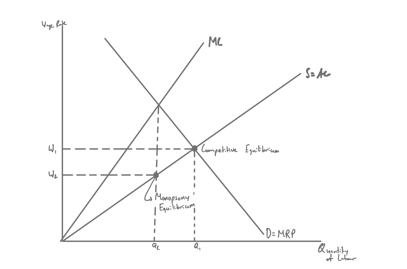
The diagram matters because it shows that monopsony is both a wage issue and an employment issue. The supply curve S = AC is the average cost of labour, and the MC curve lies above it. The competitive outcome is W1 and Q1, where D = MRP crosses S = AC, but the monopsonist hires only Q2 where MC meets D = MRP and then pays W2 from the supply curve. Workers are paid less than in a competitive market, and fewer of them are hired.

Trade unions can push back against employer power. They may bargain collectively for a higher wage, or they may restrict labour supply through membership rules, qualifications, or other barriers to entry. Union power in the UK has weakened over time because of deindustrialisation and globalisation, but also because legislation has tightened rules through postal-ballot requirements, restrictions on picketing, 14 days' notice before strikes, and turnout thresholds such as those in the Trade Union Act 2016. The Employment Rights Act 2025 has begun to relax some of these rules: since 18 February 2026, unions must give 10 days' notice of industrial action rather than 14, and the extra 40% support threshold for strikes in important public services has gone, while the 50% turnout threshold is due to be repealed later.

In a bilateral monopoly, the final wage is not pinned down by a single automatic equilibrium in the same way as a competitive market. Instead, it depends on bargaining strength. In a recession, high unemployment weakens the union's position and wages may stay closer to the monopsony level. In a boom, labour shortages strengthen workers' bargaining power and wages may move closer to, or above, the competitive level.

This is why trade unions do not always reduce employment in the simple textbook way. If a union is bargaining against a monopsonist, pushing wages up can move the market closer to the competitive outcome. In that case, both wages and employment can rise relative to the pure monopsony position.

Labour Market Frictions

Even when wage signals exist, workers do not move perfectly between jobs and places. That helps explain why the UK can have unemployment at the same time as unfilled vacancies.

When occupational mobility is low, workers cannot easily switch into the jobs where demand is strongest. Skills shortages in engineering, healthcare, and digital industries often persist because the unemployed do not automatically have the right training, qualifications, or experience. Retraining takes time and money, and some professional barriers are deliberately strict.

When geographical mobility is low, workers may know where jobs are available but still be unable or unwilling to move. High housing costs, family ties, moving expenses, and weak transport links all matter. That is why some regions can face shortages while others still have spare labour.

These frictions show up in several current labour-market issues. Young workers are often hit hardest in recessions because firms prefer to retain experienced staff and delay taking on new entrants. Missing out on work early can create wage scarring, where earnings remain lower for years afterwards.

The gig economy has also changed how labour is supplied. Firms such as Uber and Deliveroo offer flexibility, but many workers face insecurity, weaker protection, and less predictable income. Employment status decides which protections apply: in February 2021 the UK Supreme Court ruled that Uber drivers are workers, entitled to the minimum wage and paid holiday, but in November 2023 it ruled that Deliveroo riders are self-employed, so they have no such guarantee. Zero-hour contracts create a similar trade-off: employers gain flexibility, while workers face uncertainty over weekly hours and pay.

Wage inequality is another important issue. From the late 1970s, higher earners saw faster pay growth than lower earners, widening the gap between top and bottom. ONS data show that between 1997 and 2011 the top 10% of earners were paid around four times as much per hour as the bottom 10%. The gap in hourly pay has narrowed since then, to around three times by 2024, as the minimum wage has pushed up the lowest wages. At the same time, an ageing population can reduce growth in the working-age labour force and increase pressure on public finances as more people retire. Migration can ease labour shortages by increasing labour supply, but post-Brexit changes in migration policy have also left sectors such as care, agriculture, and hospitality struggling to recruit.