1.2.8 - Consumer and producer surplus
Consumer and producer surplus measure the extra benefit created when a market exchange takes place. They help economists move beyond "price went up" or "price fell" and ask a better question: who gained, who lost, and what happened to total welfare?
Why Exchange Creates Surplus
At equilibrium, the market settles at a price P* and quantity Q*. But the equilibrium price is not the highest price every buyer would have paid, and it is not the lowest price every seller would have accepted. That gap is why exchange creates surplus.
[DIAGRAM: asset_name: 1.2.8 - Consumer and producer surplus - diagram 1; asset_slug: 1.2.8 - 1; recommended_method: retained_png; description: Retained source diagram supporting 1.2.8 - Consumer and producer surplus; the packaged PNG preserves the original educational visual.]
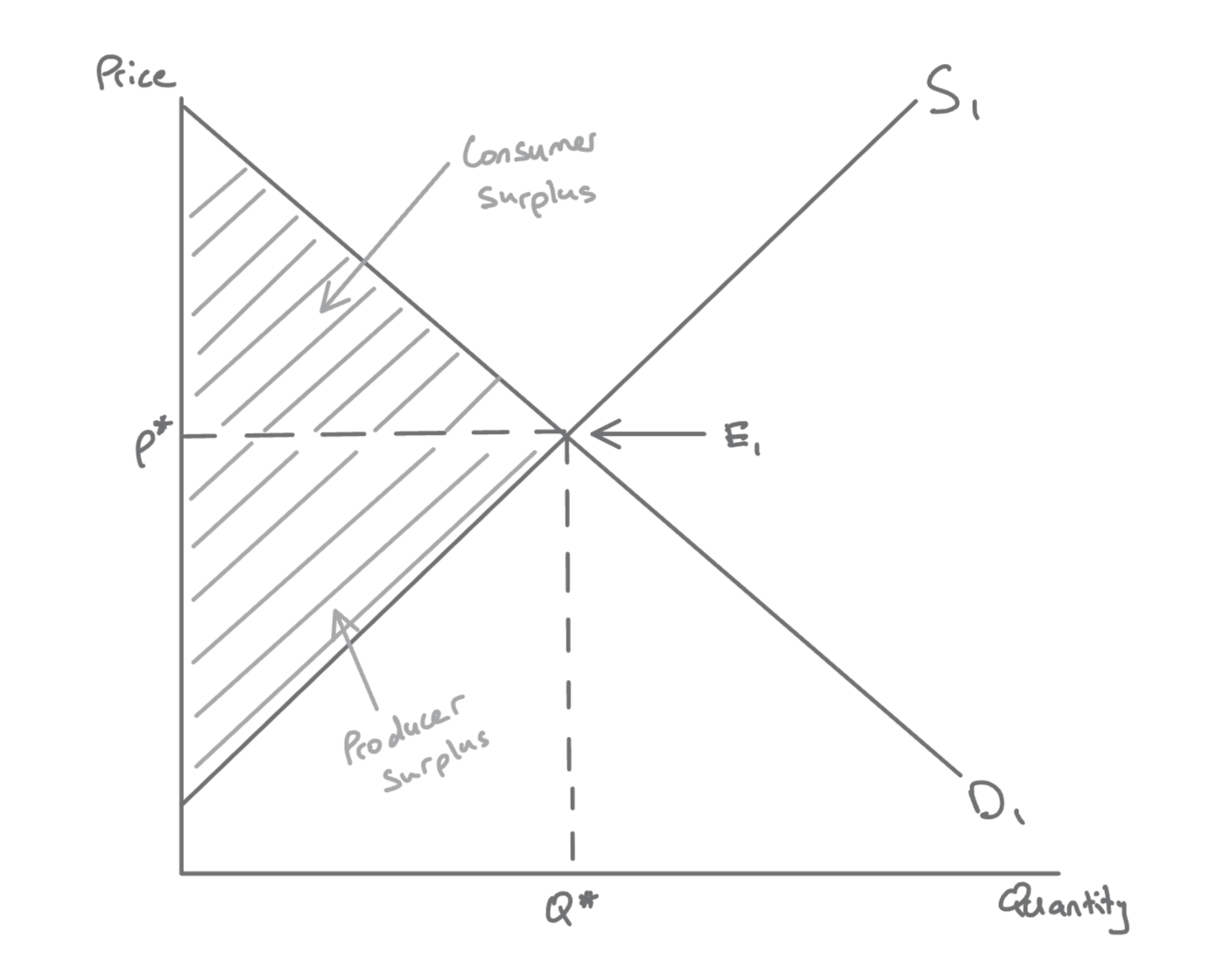
At equilibrium E1, D1 and S1 meet at P* and Q*, so the shaded triangle below D and above the price line shows consumer surplus, while the shaded triangle above S and below the price line shows producer surplus. The demand curve can be read as consumers' willingness to pay for each successive unit. The supply curve can be read as the minimum price needed to bring each successive unit to market. So the diagram is not just showing price and quantity. It is also showing the extra benefit that buyers and sellers receive from trading at the equilibrium price.
The area above the price line and below demand is consumer surplus. The area below the price line and above supply is producer surplus. Together, those two areas show the welfare created by exchange in this market.
Consumer Surplus
Definition: Consumer surplus
The difference between the price a consumer is willing and able to pay and the price they actually pay.
Suppose a student would have paid GBP4 for a coffee but buys it for GBP2.50. The student gains GBP1.50 of consumer surplus. They get something worth GBP4 to them, but only give up GBP2.50.
On the diagram, consumer surplus is the area under the demand curve and above the market price up to Q*. The area under demand shows total willingness to pay. Consumers actually spend P* x Q*. The difference between those two areas is the surplus they keep.
Because of diminishing marginal utility, each extra unit usually gives less additional satisfaction than the last. That is why willingness to pay falls as quantity rises. The marginal consumer, who is only just willing to buy at the market price, receives no consumer surplus at all. Their valuation is exactly equal to the price.
Advance rail tickets on routes such as Manchester to London often create consumer surplus. A passenger may have been willing to pay more to make the journey, but if they secure a lower advance fare, the difference is consumer surplus.
Producer Surplus
Definition: Producer surplus
The difference between the price producers receive and the minimum price at which they would be willing to supply a good.
If a bakery would have supplied one loaf for as little as GBP1.20 but sells it for GBP1.80, it gains GBP0.60 of producer surplus on that unit.
On the diagram, producer surplus is the area above the supply curve and below the market price up to Q*. In this context, the supply curve shows the minimum price needed to supply each extra unit, so it can be read as the producer's marginal cost or reservation price.
The marginal producer on the last unit sold receives no surplus on that final unit because the market price is just enough to make supply worthwhile. All the earlier units, which could have been supplied at lower prices, generate producer surplus.
Producer surplus is related to profitability, but it is not exactly the same as accounting profit. It is the extra return above the minimum supply price, shown by the triangle above supply and below price. Because the supply curve reflects marginal cost, fixed costs such as rent are not deducted, so in the short run a firm can earn producer surplus and still make a loss.
Total Welfare
When consumer surplus and producer surplus are added together, we get the total welfare created by market exchange. In a simple competitive market with no externalities, this total is maximised at the equilibrium quantity.
Formula: Surplus and welfare
Worked example: with straight-line demand and supply, each surplus is a triangle, so its area is 1/2 x base x height. Suppose a cinema's equilibrium is GBP8 a ticket and 2,000 tickets a week. The highest willingness to pay, where demand meets the price axis, is GBP14, and the minimum price needed to supply the first ticket is GBP4.
Why does equilibrium maximise total welfare? If output were below Q*, there would still be units for which consumers value the good more than it costs producers to supply, so mutually beneficial trades are being missed. If output were above Q*, some extra units would cost more to supply than consumers are willing to pay, so those units reduce welfare rather than add to it. Only at Q* does the value of the last unit to consumers exactly equal the marginal cost of supplying it.
Exam tip
Surplus analysis is mainly about efficiency, not fairness. A market can create large total welfare and still distribute it unequally. The exact size of the surplus areas also depends on elasticity, and price discrimination changes the split because consumers no longer all pay the same market price.
Do not treat every fall in consumer or producer surplus as deadweight loss. In tax, subsidy, and price-control questions, part of the lost surplus may simply be transferred to another group, such as producers or the government. Deadweight loss is only the welfare from mutually beneficial trades that no longer happen.
This is why consumer and producer surplus matter beyond one diagram. The same framework is used later to analyse taxes, subsidies, price controls, and market failure.
How Surplus Changes
Because surplus depends on both price and quantity, it changes when demand or supply changes.
When demand increases, price and quantity both rise. Producer surplus rises because firms sell more units at a higher price. Consumer surplus usually rises as well because consumers are willing to pay more and more units are bought, although the higher price offsets part of that gain. When demand decreases, producer surplus falls and consumer surplus usually falls, though the lower price partly cushions the effect for remaining buyers.
When supply increases, price falls and quantity rises. Consumer surplus rises because buyers pay less and more consumers enter the market. Producer surplus often rises too if the rightward shift reflects lower costs or improved productivity. When supply decreases, consumer surplus falls, but producer surplus is ambiguous: firms receive a higher price, yet they sell fewer units and are often facing higher costs. Which effect is larger depends mainly on the price elasticity of demand: the more inelastic demand is, the more price rises and the less quantity falls, so the better producers fare. With very inelastic demand, producers who still have output to sell, such as farmers after a poor harvest, can even gain.
[DIAGRAM: asset_name: 1.2.8 - Consumer and producer surplus - diagram 2; asset_slug: 1.2.8 - 2; recommended_method: retained_png; description: Retained source diagram supporting 1.2.8 - Consumer and producer surplus; the packaged PNG preserves the original educational visual.]
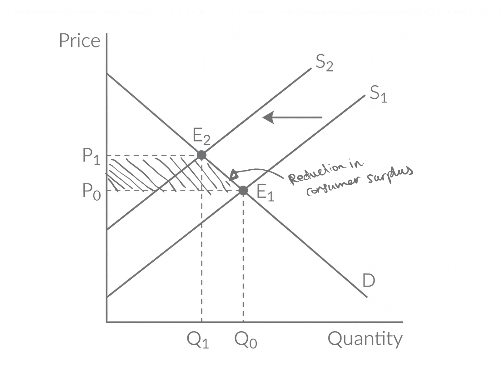
With D fixed, the leftward shift from S1 to S2 moves the market from E1 at P0, Q0 to E2 at P1, Q1, so consumer surplus shrinks and producer surplus becomes ambiguous. The shaded area between P0 and P1, to the left of D, is the lost consumer surplus. It has two parts: a rectangle, because buyers who still purchase Q1 now pay P1 instead of P0, and a small triangle between Q1 and Q0, from trades that no longer happen. Read the diagram in reverse, from S2 to S1, and it shows a supply increase: price falls from P1 to P0, quantity rises from Q1 to Q0, and consumer surplus grows by the same shaded area. In the UK strawberry market, a good summer harvest shifts supply to the right. Supermarkets can sell more punnets at a lower price, so consumer surplus rises. Producer surplus may also rise if growers can sell many more punnets at lower unit cost. This happened in 2025: after the UK's warmest and sunniest spring on record, an early glut of British strawberries let Tesco cut its 400g punnets from GBP2.50 to GBP1.50 and expect to sell about a quarter more than the year before.
A useful exam drill is to classify the direction of change first, before you start evaluating the size of the change:
| Change | Price | Quantity | Consumer surplus | Producer surplus |
|---|---|---|---|---|
| Demand increases | Up | Up | Usually up | Up |
| Demand decreases | Down | Down | Usually down | Down |
| Supply increases | Down | Up | Up | Usually up |
| Supply decreases | Up | Down | Down | Ambiguous |
Once you can classify the direction of change, the next step in an exam answer is to explain the causal chain clearly in context.
Quick Recap
- Consumer surplus is the gap between willingness to pay and the market price.
- Producer surplus is the gap between the market price and the minimum price needed to supply.
- In a simple competitive market, total welfare is the sum of both surpluses and is maximised at equilibrium.
- Demand and supply shifts redistribute surplus, and a fall in supply is the classic case where producer surplus becomes ambiguous.