2.4.3 - Equilibrium levels of real national output

Equilibrium in the Short Run

Both Classical and Keynesian economists start from the same short-run picture. Aggregate demand slopes downward, short-run aggregate supply slopes upward, and the equilibrium level of real national output is found where the two curves intersect.

AD includes consumption, investment, government spending, and net exports. If the general price level is lower, spending is usually higher in real terms, so the AD curve slopes down from left to right. Three effects explain this: lower prices raise the real value of households' cash and savings (the real balances or wealth effect), tend to reduce interest rates (the interest rate effect), and make domestic goods more competitive against foreign ones (the international competitiveness effect).

SRAS slopes upward because higher prices can make it more worthwhile for firms to expand output while some costs are still fixed or slow to adjust.

[DIAGRAM: asset_name: 2.4.3 - Equilibrium levels of real national output - diagram 1; asset_slug: 2.4.3 - 1; recommended_method: retained_png; description: Retained source diagram supporting 2.4.3 - Equilibrium levels of real national output; the packaged PNG preserves the original educational visual.]

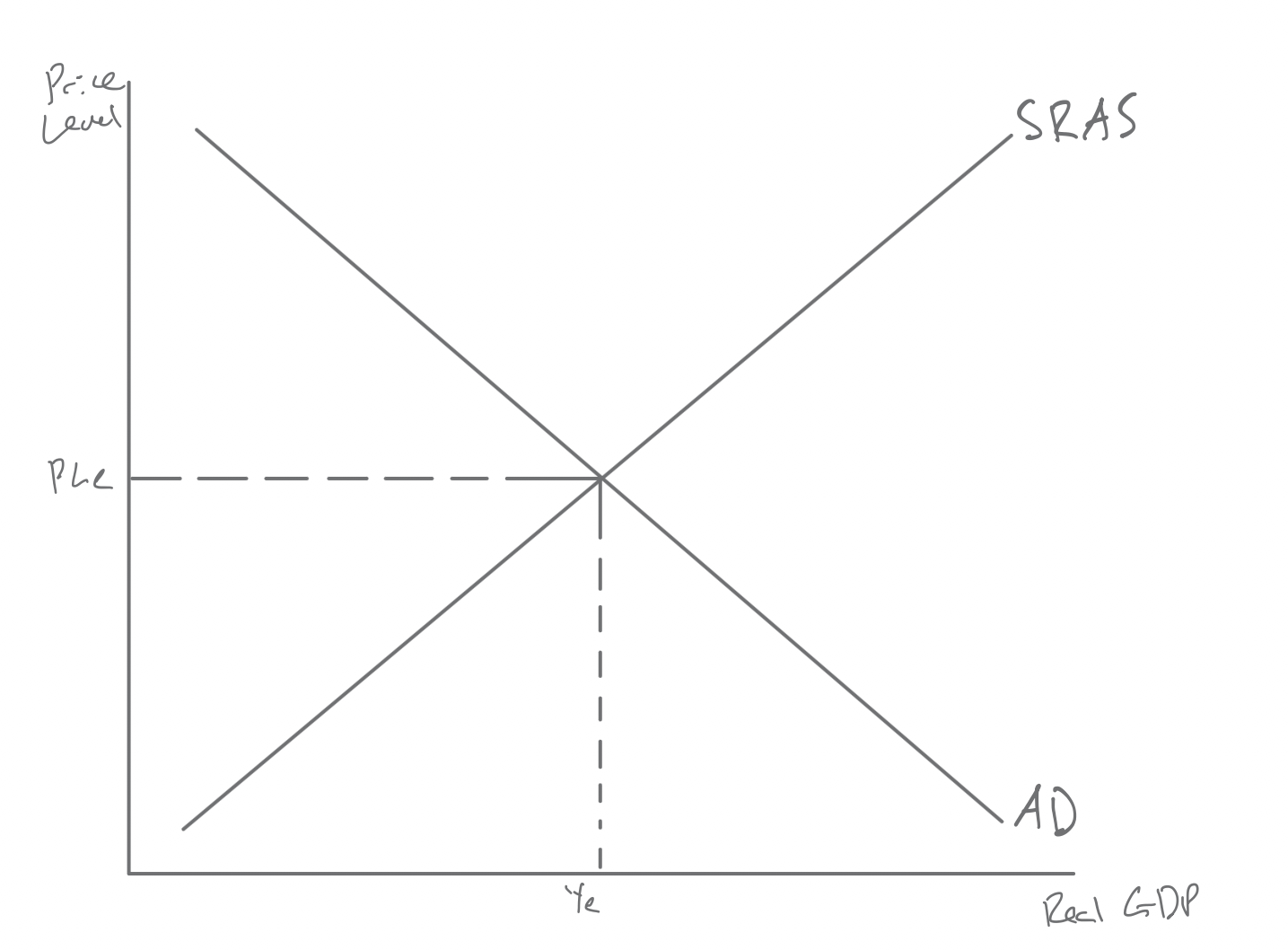
In the diagram, AD and SRAS intersect at the equilibrium price level PLe and the equilibrium level of real GDP Ye.

At the intersection of AD and SRAS, firms are selling what they planned to produce. There is no unplanned build-up of stocks, no unplanned depletion of inventories, and no immediate reason for firms to expand or cut output. For the moment, there is also no pressure for the general price level to move away from that equilibrium point.

Away from that point, the economy is pushed back towards it. Above PLe, firms plan to supply more than households, firms, the government and foreign buyers plan to buy, so unsold stocks build up and firms cut output and prices. Below PLe, planned spending is greater than planned output, so inventories run down and firms raise output and prices until spending and output match again.

One important caveat is that equilibrium does not automatically mean full employment. The economy can be in equilibrium with spare capacity if AD is weak, and it can also move temporarily above its sustainable level if AD becomes too strong.

When Demand or Supply Changes

When AD changes, equilibrium output and the price level both change in the short run. A rightward shift in AD might be caused by higher consumer confidence, stronger business investment, more government spending, or an improvement in net exports. The new equilibrium normally has higher real output and a higher price level. A leftward shift in AD causes the opposite: lower output and a lower price level. To show any of these changes on an AD/AS diagram, draw the new curve, mark where it intersects the unchanged curve, and label the new equilibrium price level and real output on the axes.

How far output rises depends on how much spare capacity the economy has and how elastic aggregate supply is. If many workers and machines are sitting idle, firms can respond to extra demand by producing more. If the economy is already close to capacity, the same increase in AD is more likely to push up prices than output.

Changes in SRAS produce a different pattern. If wages rise, raw material costs increase, or indirect taxes go up, SRAS shifts left. Firms are willing to supply less at each price level, so equilibrium output falls while the price level rises. That awkward combination of weaker output and higher inflation is called stagflation. The 1973-74 oil shock is the classic case: the price of crude oil roughly quadrupled, raising costs across the economy, and the UK fell into recession while inflation rose above 20% in 1975. If SRAS shifts right because costs fall or productivity improves, the economy gets the more favourable result of higher output and lower prices.