4.9 - Sketching curves with known turning points
Build a reliable curve sketch from its known maximum and minimum points, axis intercepts and far-end behaviour. You will distinguish crossings from touches and use the finished shape to interpret gradients and count solutions without inventing coordinates.
Building a cubic sketch from its anchors
Can a cubic have two turning points but only two different -intercepts? A familiar S-shaped curve often has three crossings, but one of its turns can change that count. We will reach that case after assembling a complete ordinary cubic sketch.
You already know
Set for -intercepts and for the -intercept. A maximum has a horizontal tangent with rising then falling behaviour; a minimum has falling then rising behaviour. A sketch shows correct features and their order rather than a table of accurately plotted points.
Use the supplied turning points as anchors. If their coordinates and natures are given, you can use them directly; there is no need to repeat the calculus unless the question asks you to establish them. Place them and the intercepts before joining anything.
The leading term controls a polynomial's far ends, where its highest power dominates the lower powers. For example, a positive term eventually gives negative outputs far to the left and positive outputs far to the right.
Polynomial far-end behaviour
For a nonconstant polynomial with leading term , where and is a positive integer,
“Far ends” describes behaviour for very large positive or negative inputs, not the direction at every point.
Not on the formulae sheet: learn it.
Connect the anchors with a smooth curve that respects those ends and the given turns. Do not insert another turn merely to make the sketch look tidy.
Worked example 1: three distinct crossings
Question. The curve has a maximum at and a minimum at . Sketch it, labelling the intercepts and turning points.
Plan. Factorise for the intercepts, place the known turns and use the positive cubic term for the ends.
Why this step? The intercepts fix where the curve meets the axis; the known turns fix the rise-fall-rise route between its far ends.
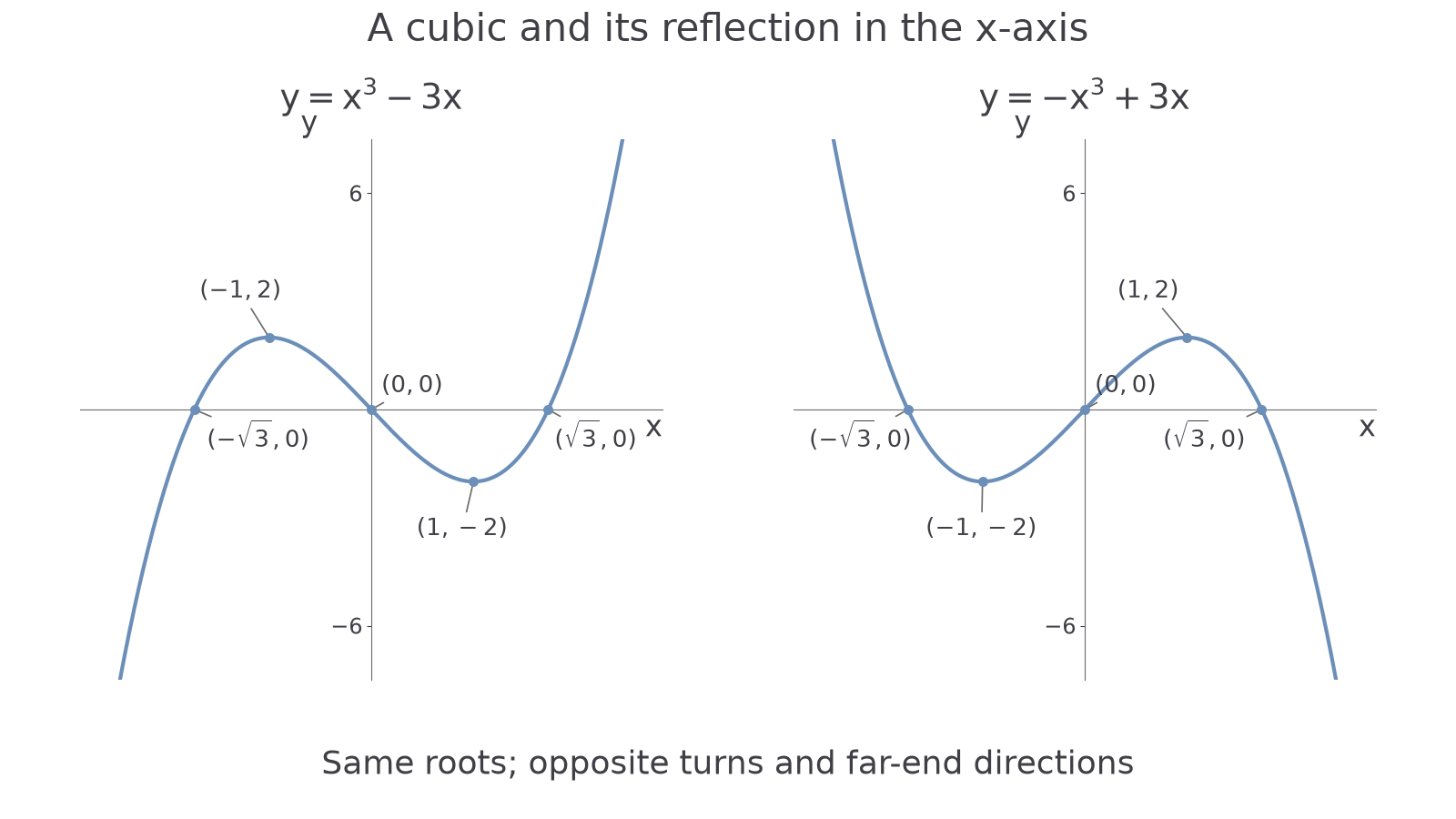
Answer. Draw a smooth cubic rising from the lower left through to the maximum, falling through to the minimum, then rising through towards the upper right. The left panel below shows the sketch.
Check. , so all labelled features occur in the stated order. The simple factors change sign at each root, so all three are crossings.
Worked example 2 multiplies the entire rule by . The roots stay fixed, while heights and end directions reverse.
Worked example 2: a negative-leading cubic
Question. The curve has a minimum at and a maximum at . Sketch it, labelling the intercepts and turning points.
Plan. Use the unchanged roots and reflected turning points, then reverse the far-end directions.
Why this step? Multiplication by reflects the whole graph in the -axis. It cannot move a point that already has height zero.
Answer. Draw a smooth cubic falling from the upper left through to the minimum, rising through to the maximum, then falling through . See the right panel below.
Check. Every point from the first sketch becomes , including both turning points and all three unchanged intercepts.
The comparison makes the leading coefficient's role visible. Both curves have the same roots and the same turning-point inputs, but travel through them in opposite directions.
[DIAGRAM: asset_name: Reflecting a complete cubic sketch; asset_slug: l2fm-cubic-sketch-reflection; caption: Multiplying by minus one preserves the roots while reversing the turns and both far ends; description: Two coordinate graphs show y equals x cubed minus 3x and y equals minus x cubed plus 3x. Both label roots at minus square root 3, zero and square root 3. The first labels maximum minus 1 comma 2 and minimum 1 comma minus 2; the second labels minimum minus 1 comma minus 2 and maximum 1 comma 2. Each curve continues in the correct far-end directions]
A sketch communicates coordinates through labels, so an accurately placed but unlabelled intercept can still leave the reader uncertain.
Watch out
Wrong: connect the anchors with straight segments or draw a sharp corner at a turning point. A smooth polynomial has a horizontal tangent there. Draw the curve smoothly through each turn.
Prepare the anchors for a new cubic without needing to draw in the answer box.
Recognising touches and repeated roots
A root does not always make the curve cross the axis: a repeated factor can make it turn back on the same side.
For , the squared factor is positive on both sides of . The other factor is also positive near , so the curve stays above the axis as it reaches and leaves that root. At , the factor changes sign while the square stays positive, so the curve crosses.
Root multiplicity and the axis
If a polynomial can be written near a root as
where is a positive integer, then an even gives a touch with no sign change, while an odd gives a crossing. The nonzero remaining factor keeps the same sign sufficiently close to .
Not on the formulae sheet: learn it.
This includes an important boundary: has a repeated root of odd multiplicity and crosses with a horizontal tangent. “Repeated” alone does not decide between a crossing and a touch.
Worked example 3: a minimum on the axis
Question. Sketch . Its maximum is and its minimum is . Label the axis intercepts and turning points.
Plan. Read the roots and their multiplicities, calculate the vertical intercept and combine them with the supplied turns.
Why this step? The known minimum lies on the axis. The curve must touch it smoothly and rise again, rather than pass below it.
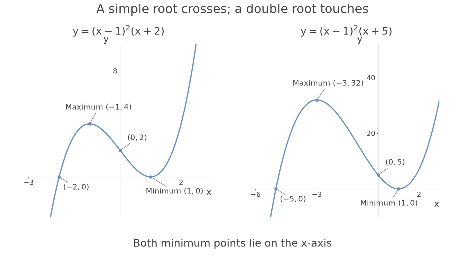
Answer. Draw a cubic crossing at , rising to , falling through to touch at , then rising. It has two distinct -intercepts, answering the opening question.
Check. Expanding gives . Its derivative is , confirming the two supplied stationary inputs.
Worked example 4 changes only the constant in the unsquared factor, from to . The double root stays at , while the other crossing and maximum move.
Worked example 4: moving the other root
Question. Sketch . Its maximum is and its minimum is . Label the axis intercepts and turning points.
Plan. Read the new simple root, retain the double root and calculate the new vertical intercept.
Why this step? Changing the other factor does not change the root of , but it changes heights away from that root.
Answer. Draw the left end down, cross at , rise to , fall through , touch at and rise to the right.
Check. Expanding gives , whose derivative is . At , the original product is .
The panels show the two sketches on suitable vertical scales. Neither curve needs a third crossing just because it is cubic.
[DIAGRAM: asset_name: Two cubic sketches with a double root; asset_slug: l2fm-cubic-double-root; caption: Both cubics cross at their simple root and touch at their shared double root; description: Two coordinate graphs show y equals open bracket x minus 1 close bracket squared times open bracket x plus 2 close bracket and the same squared factor times open bracket x plus 5 close bracket. The first labels crossing minus 2 comma 0, maximum minus 1 comma 4, vertical intercept zero comma 2 and touching minimum 1 comma 0. The second labels crossing minus 5 comma 0, maximum minus 3 comma 32, vertical intercept zero comma 5 and touching minimum 1 comma 0. Both have left end down and right end up]
The first curve hides a different kind of symmetry. If , then . Rotating the graph through about maps it onto itself. For example, pairs with , and its maximum pairs with its minimum. Cubic symmetry can be a half-turn rather than a mirror line.
Watch out
Wrong: draw every root as a crossing, or every repeated root as a touch. Check the complete factor's multiplicity: even powers preserve its sign across the root; odd powers reverse it.
The next cubic touches the axis at a maximum rather than a minimum. Use its factors to decide what happens at each root.
Continue this lesson.
You’re previewing NovaLearn without an account. Create a free account to read the rest.
Create free account