4.5 - Increasing and decreasing functions

Use a gradient function to describe where a curve rises or falls as you move to the right. You will solve derivative inequalities, prove that a function increases for every real input and handle a parameter without confusing a positive gradient with an isolated horizontal tangent.

Reading increasing and decreasing from the gradient

Can a function increase for every real input even though its gradient is zero somewhere? That sounds contradictory until you distinguish a horizontal tangent at one point from a flat stretch of graph.

Increasing and decreasing

A function is increasing on an interval if larger inputs give larger outputs: whenever $a<b$ in that interval, $f(a)<f(b)$ . It is decreasing if larger inputs give smaller outputs: $f(a)>f(b)$ . Read the graph from left to right; positive or negative heights do not decide whether it is increasing.

A positive tangent gradient means the curve is rising locally; a negative tangent gradient means it is falling locally. To establish behaviour over an interval, check the derivative's sign throughout that interval, rather than at just one convenient input.

The derivative sign test

For a differentiable function on an interval,

\frac{\mathrm{d}y}{\mathrm{d}x}>0\text{ throughout}\Longrightarrow\text{increasing}

\frac{\mathrm{d}y}{\mathrm{d}x}<0\text{ throughout}\Longrightarrow\text{decreasing}

An isolated zero gradient needs further thought; it does not by itself reverse the behaviour.
Not on the formulae sheet: learn it.

For a linear derivative, the required sign intervals come from solving a linear inequality.

Worked example 1: a linear gradient function

Question. For $y=x^2-6x+4$ , work out where the gradient is positive and where it is negative. State the function's behaviour on those intervals.

Plan. Differentiate, then solve the positive and negative derivative inequalities.

\begin{aligned} \frac{\mathrm{d}y}{\mathrm{d}x}&=2x-6 &&\text{differentiate}\\ 2x-6>0&\Longrightarrow x>3 &&\text{positive gradient}\\ 2x-6<0&\Longrightarrow x<3 &&\text{negative gradient} \end{aligned}

Why this step? The derivative controls the direction of change; solving $y>0$ would instead describe where the curve is above the axis.

Answer. Positive gradient and increasing for $x>3$ ; negative gradient and decreasing for $x<3$ . The gradient is zero at $x=3$ .

Check. At $x=2$ , the derivative is $-2$ ; at $x=4$ , it is $2$ , agreeing with the two intervals.

Change only the coefficient of $x^2$ , from $+1$ to $-1$ . When you divide the new inequalities by a negative number, reverse their direction.

Worked example 2: reversing an inequality

Question. For $y=-x^2-6x+4$ , work out where the gradient is positive and where it is negative. State the function's behaviour there.

Plan. Differentiate and solve the sign inequalities, taking care with division by $-2$ .

\begin{aligned} \frac{\mathrm{d}y}{\mathrm{d}x}&=-2x-6 &&\text{differentiate}\\ -2x-6>0&\Longrightarrow-2x>6\Longrightarrow x<-3 &&\text{reverse on division}\\ -2x-6<0&\Longrightarrow-2x<6\Longrightarrow x>-3 &&\text{reverse again} \end{aligned}

Why this step? Dividing an inequality by a negative number reverses which side is greater; the calculus has not changed that algebra rule.

Answer. Positive gradient and increasing for $x<-3$ ; negative gradient and decreasing for $x>-3$ . The gradient is zero at $x=-3$ .

Check. At $x=-4$ , the derivative is $2$ ; at $x=-2$ , it is $-2$ .

The reported intervals use strict inequalities because the question asks where the gradient is positive or negative. Including an endpoint with zero gradient can still be compatible with the function increasing or decreasing on the resulting interval.

Watch out

Wrong: a function is decreasing wherever $y<0$ . The sign of $y$ gives height, not direction. For example, $y=x-100$ is negative at $x=1$ , but its gradient is $1$ , so it is increasing.

Use a new linear derivative to report both behaviours.

Solving a quadratic gradient inequality

A quadratic derivative can change sign twice. Factorise it, identify its zeros and use the signs of its factors to describe the intervals between them.

[DIAGRAM: asset_name: Derivative signs along a cubic; asset_slug: l2fm-increasing-decreasing; caption: The curve rises, falls, then rises as its derivative changes from positive to negative to positive; description: A blue curve y equals x cubed minus 3x is shown on coordinate axes, with vertical dashed guides at x equals minus 1 and x equals 1. Pale sage bands outside these values show positive derivative 3x squared minus 3 and increasing behaviour. A pale clay band between them shows negative derivative and decreasing behaviour. A separate aligned sign strip records plus, zero, minus, zero, plus]
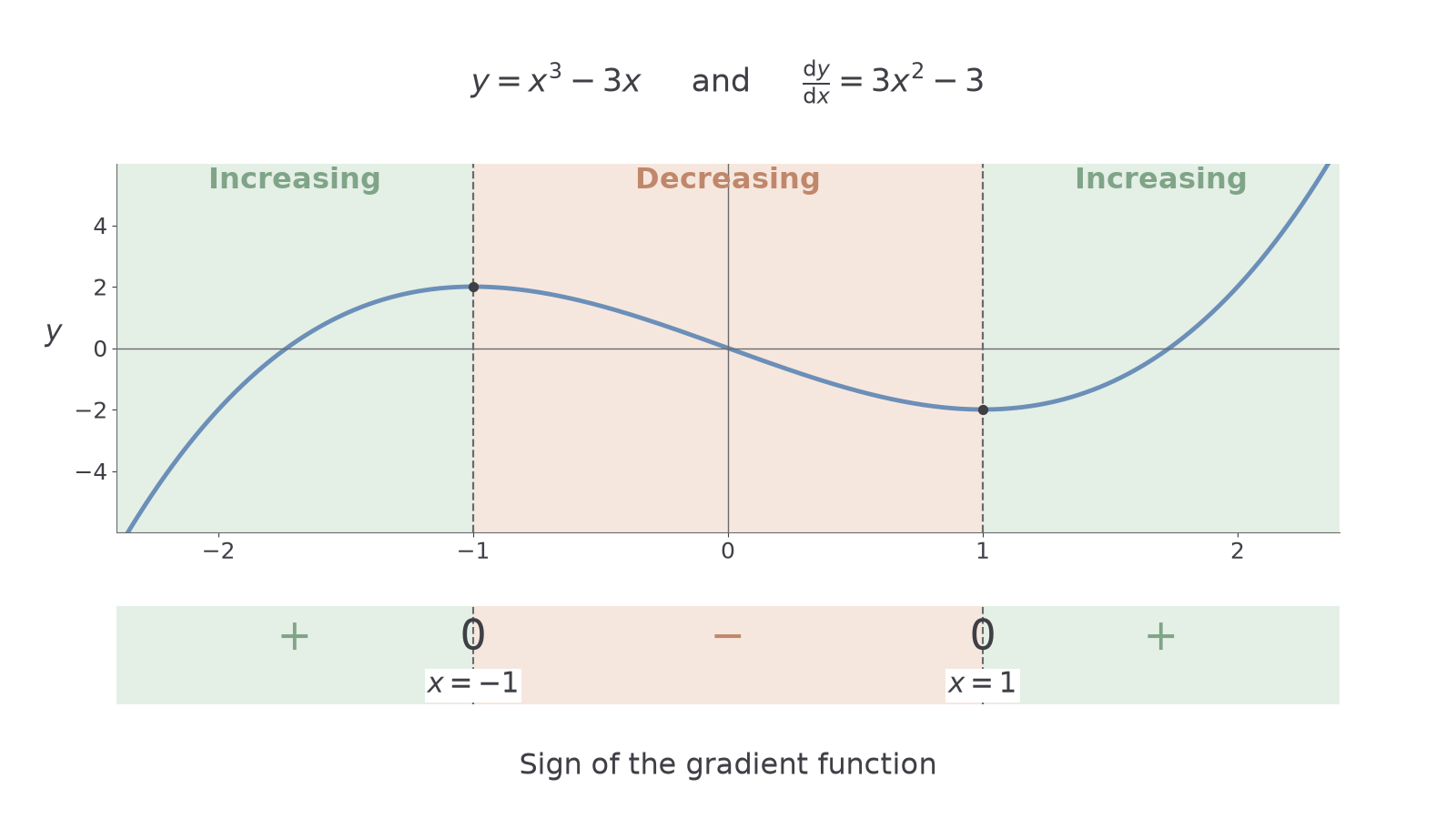
The curve rises, falls, then rises as its derivative changes from positive to negative to positive

The zeros divide the real line into intervals. A continuous polynomial derivative cannot change sign inside one of those intervals without passing through another zero, so testing one point per interval is enough after all its zeros are known.

Worked example 3: two derivative zeros

Question. For $y=x^3-3x$ , work out where the derivative is positive or negative and state the function's behaviour there.

Plan. Differentiate, factorise, then check the signs outside and between the zeros.

\begin{aligned} \frac{\mathrm{d}y}{\mathrm{d}x}&=3x^2-3=3(x-1)(x+1) &&\text{differentiate and factorise}\\ \frac{\mathrm{d}y}{\mathrm{d}x}=0&\Longrightarrow x=-1\text{ or }x=1 &&\text{interval boundaries}\\ 3(x-1)(x+1)>0&\Longrightarrow x<-1\text{ or }x>1 &&\text{factors have matching signs}\\ 3(x-1)(x+1)<0&\Longrightarrow-1<x<1 &&\text{factors have opposite signs} \end{aligned}

Why this step? A positive leading coefficient makes this quadratic derivative positive outside its two roots and negative between them.

Answer. Increasing for $x<-1$ and $x>1$ , where the derivative is positive; decreasing for $-1<x<1$ , where it is negative.

Check. At $x=-2,0,2$ , the derivative values are $9,-3,9$ , giving the sign pattern shown in the diagram.

Change only the coefficient of the linear term from $-3$ to $-12$ . The derivative's zeros move, but its sign pattern stays the same.

Worked example 4: new boundaries, same sign pattern

Question. For $y=x^3-12x$ , work out where the derivative is positive or negative and state the function's behaviour there.

Plan. Factorise the new derivative and use its two roots to divide the real line.

\begin{aligned} \frac{\mathrm{d}y}{\mathrm{d}x}&=3x^2-12=3(x-2)(x+2) &&\text{differentiate and factorise}\\ \frac{\mathrm{d}y}{\mathrm{d}x}=0&\Longrightarrow x=-2\text{ or }x=2 &&\text{new boundaries}\\ \frac{\mathrm{d}y}{\mathrm{d}x}>0&\Longrightarrow x<-2\text{ or }x>2 &&\text{outside the roots}\\ \frac{\mathrm{d}y}{\mathrm{d}x}<0&\Longrightarrow-2<x<2 &&\text{between the roots} \end{aligned}

Why this step? Solving the equation gives only the boundaries. The inequalities are what identify whole intervals of increasing or decreasing behaviour.

Answer. Increasing for $x<-2$ and $x>2$ ; decreasing for $-2<x<2$ , with positive and negative derivative respectively.

Check. At $x=-3,0,3$ , the derivative values are $15,-12,15$ , again positive, negative, positive.

Knowing the sign pattern is more useful than just listing the derivative zeros.

Watch out

Wrong: the function is increasing “at $x=-2,2$ ” because those solve $\frac{\mathrm{d}y}{\mathrm{d}x}=0$ . Those are zero-gradient inputs. The positive-gradient regions are the intervals outside them.

The next linear coefficient moves the boundaries again. Give complete intervals rather than a list of roots.

Continue this lesson.

You’re previewing NovaLearn without an account. Create a free account to read the rest.

Create free account

Last Accessed

Number

Algebra

Coordinate geometry

Calculus

Matrix transformations

Geometry

4.5 - Increasing and decreasing functions

Reading increasing and decreasing from the gradient

Solving a quadratic gradient inequality

Continue this lesson.

Learn faster with Nova