Appendix 4 - Summarising data and judging relationships

Choosing a representative value

The mean is the total divided by the number of observations. The median is the middle value after ordering the observations; with an even number, average the two middle values. The mode is the most frequent value; there can be several modes or none. For grouped continuous data, the modal class is the interval with greatest frequency when equal-width classes are used.

Consider these simulated river depths in centimetres: 10, 12, 12, 14, 17. Their mean is 65/5 = 13 cm, median 12 cm and mode 12 cm. Add a 55 cm reading and the mean becomes 120/6 = 20 cm, while the median becomes (12+14)/2 = 13 cm. The deep reading may be a real pool rather than a mistake. Investigate it; do not delete a value merely because it changes the story.

The mean uses all values and is useful for many physical totals/averages, but an extreme value can pull it away from most observations. The median resists that pull but does not describe the size of every difference. The mode can summarise a category such as the most common travel mode, where averaging category names makes no sense. State which measure you use and why it fits the question.

Spread, quartiles and cumulative frequency

The range is maximum minus minimum; it depends on only two values. Quartiles divide an ordered distribution into quarters. The lower quartile Q1 is near the 25th percentile, the median near the 50th and the upper quartile Q3 near the 75th. The interquartile range (IQR) is Q3 − Q1: the spread of the middle half, less affected by extremes than the full range.

For the ordered values 2, 4, 5, 7, 9, 10, 12, 15, use the median-of-halves convention: median 8, Q1 = (4+5)/2 = 4.5, Q3 = (10+12)/2 = 11, so IQR = 6.5 and range = 13. Different software/texts can interpolate quartiles differently in a small dataset. State the convention or use the method supplied with the question rather than treating all alternatives as careless arithmetic.

A cumulative frequency total accumulates observations up to a boundary. For classes 0–<10, 10–<20, 20–<30, 30–<40 with frequencies 2, 5, 8, 5, cumulative totals at the upper boundaries are 2, 7, 15, 20. Plot the boundaries against these totals, starting at (0,0). To estimate the median for 20 observations, go across from cumulative frequency 10 to the curve, then down to diameter: about 24 mm if values are spread evenly within the 20–30 class. Grouping loses the original positions, so this is an estimate.

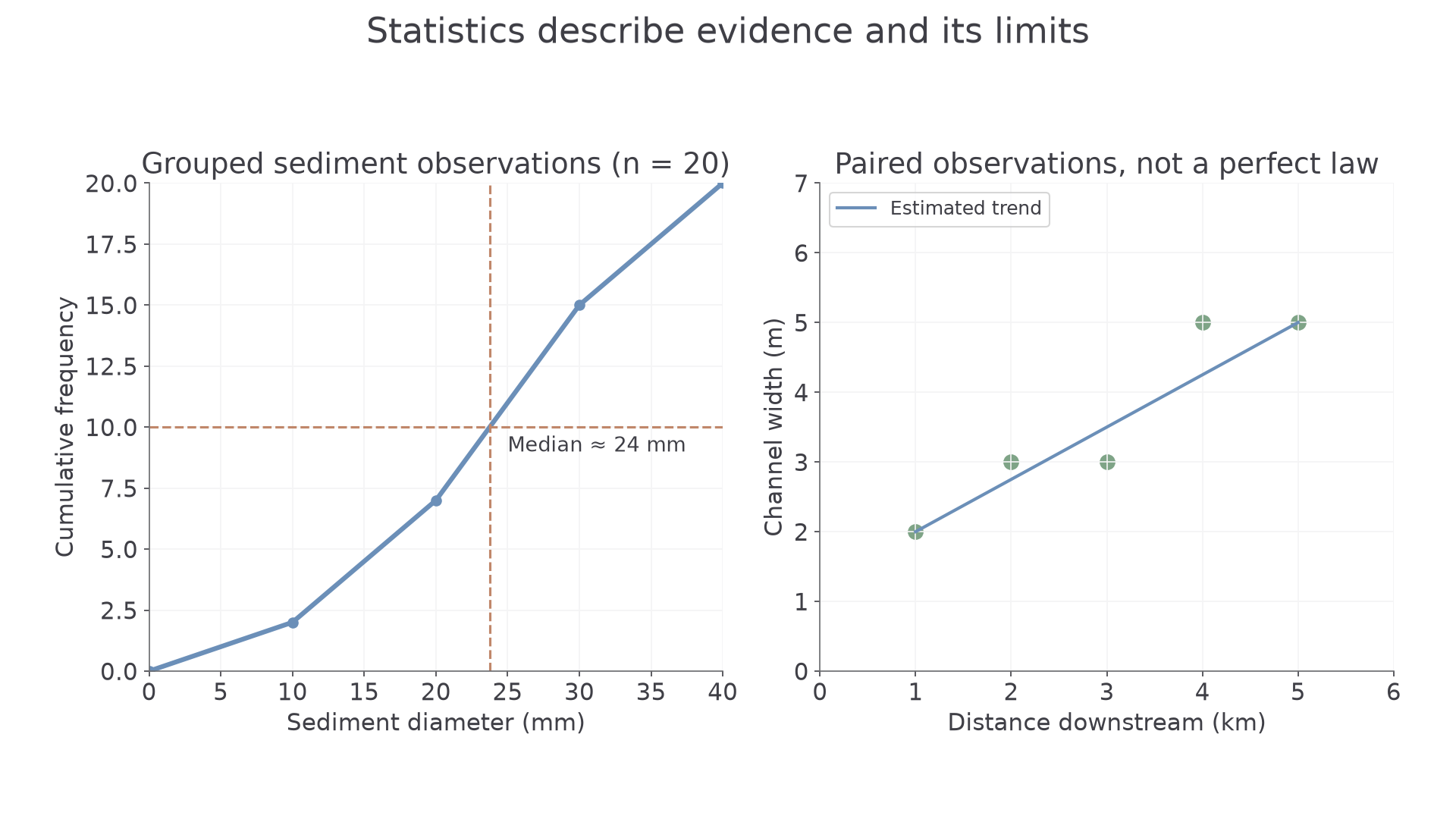
Original simulated data. The cumulative graph estimates values within groups; the scatter shows a trend with local departures rather than a perfect physical law.

A 90th percentile is a value with approximately 90% of observations at or below it. It is a position, not a 90% increase. Always check whether larger numbers represent better or worse outcomes before interpreting a high percentile.

Relationships, predictions and anomalies

Bivariate data contain paired values of two variables for each observation. A scatter pattern rising from left to right suggests positive correlation; a falling pattern suggests negative correlation. Tight clustering around a trend suggests a stronger relationship than widely scattered points. “Strong” describes consistency, not whether the slope is steep.

Draw an estimated line of best fit through the main pattern, with points reasonably balanced around it. It need not pass through the origin or every point. Use the trend only where a prediction is meaningful. Interpolation estimates within the observed range; extrapolation extends beyond it and is more uncertain because the relationship may change. A river cannot widen indefinitely just because several upstream sites show increasing width.

A simulated set gives downstream distances 1, 2, 3, 4, 5 km and widths 2, 3, 3, 5, 5 m. A rough trend predicts around 4 m at 3.5 km. Predicting at 20 km reaches far beyond the observations: a dam, tributary or different geology could alter the channel. A point away from the trend is an anomaly, not automatically an error. Recheck the record, then examine a possible local explanation.

Correlation alone does not prove causation. Towns with more shops may also have more traffic because both relate to population size. A defensible explanation needs a mechanism and evidence that competing influences do not better explain the pattern.

Recognising selective presentation

Statistics can be accurate individually yet misleading together. Compare the claim with the evidence that was selected. A graph beginning just before an unusually low year can exaggerate later growth. A truncated bar axis can magnify a small difference. A mean without spread can conceal large inequalities, while an area average can hide neighbourhood contrasts.

Denominators matter. “80% support” means different things if four of five volunteers responded or 800 of 1000 randomly selected households did. A larger volunteer sample may still exclude important groups. Do not average site percentages without checking sample sizes: 90% of 10 and 10% of 90 combine to 18% overall, not 50%. There are 9 + 9 = 18 supporters out of 100.

Look for missing comparisons, definitions and source dates. Ask whether the same boundaries, categories, time intervals and measurement methods were used. A careful conclusion acknowledges a limitation and says how it affects confidence; it does not reject every statistic because all data have limits.