1.4 - River fieldwork: analysing channel evidence
Apply 1.4 analysis and evaluation to river measurements, sketches and GIS evidence. Work from patterns to a bounded conclusion, then test whether the methods really support it.
Processing and presenting channel data
Processing makes field records comparable without erasing their context. Convert units, preserve repeats, calculate suitable means and record missing readings. Width/depth describe channel form; velocity describes water movement. Greater width alone does not prove greater discharge because depth and mean velocity also matter.
The following original simulated records are for a 2 km reach, not a student's completed fieldwork. Each depth/velocity is the mean of several readings; its sampling method still needs evaluation.
| Site | Distance downstream (km) | Wetted width (m) | Mean depth (m) | Mean velocity (m/s) | Channel fall over 100 m (m) |
|---|---|---|---|---|---|
| A | 0 | 2.0 | 0.20 | 0.30 | 2.0 |
| B | 1 | 3.0 | 0.30 | 0.55 | 1.0 |
| C | 2 | 4.0 | 0.35 | 0.50 | 0.5 |
Width increases by 2 m from A to C, a 100% increase from its 2 m baseline. Approximate cross-sectional areas are 0.40, 0.90 and 1.40 m²; estimated discharges are 0.12, 0.495 and 0.70 m³/s. These calculations rely on representative depths/velocities. Round at the end and do not imply greater precision than the instruments support.
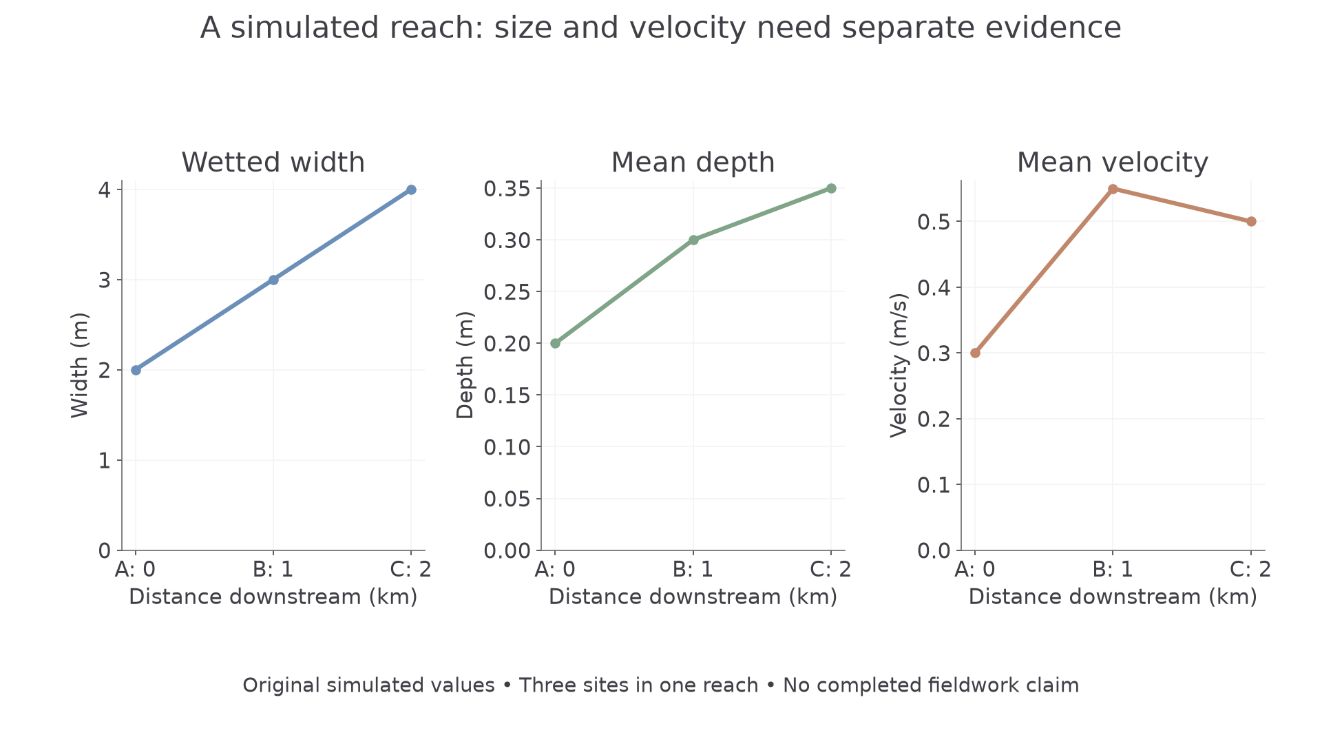
Original training values. The figures show increasing channel size but a local velocity fall between B and C.
A cross-section graph shows how depth varies across a channel; a scatter/line plot compares a measured variable with downstream distance. A GIS map locates the pattern and can combine primary site points with secondary topography. Choose by the question: a graph shows values precisely, while the map can reveal the tributary or land-use context behind them.
Connecting primary and secondary evidence
A GIS topographic dataset for this simulated reach records elevations A 120 m, B 110 m and C 105 m, a tributary entering before B and an engineered wide section at C. A distinct local flow archive records that survey-day flow was above that month's median. An annotated field sketch at C records a broad shallow margin with reeds; the sketch cannot independently measure its velocity.
These sources answer different questions. Relief supports the downstream direction and a flattening long profile. The tributary offers a mechanism for increased discharge by B. The engineered section and vegetation could help explain why mean velocity falls slightly at C despite increasing channel area. Above-median flow warns that the measurements may not represent a typical low-flow day. Neither the map nor the archive directly measures the exact survey cross sections.
Check spatial and temporal alignment: a gauge elsewhere in the catchment may respond differently, old mapping may omit management, and a coarse GIS layer may simplify a narrow channel. A useful secondary source supports a specific inference; writing “I used the internet” does not explain its contribution.
Continue this lesson.
You’re previewing NovaLearn without an account. Create a free account to read the rest.
Create free account