Appendix 4 - Relief, transects and GIS evidence

Contours and changes in height

Relief is the shape and variation in height of the land. A contour joins points of equal elevation above a stated datum, usually mean sea level. A spot height gives the elevation of one point. Read the contour interval: five closely spaced 20 m contours indicate a steeper slope than the same height change spread over a longer horizontal distance. Wide spacing alone does not reveal the height; a broad plateau can be high and gently sloping.

Closed contours with rising values towards the centre indicate a hill. A valley's contours often make a V pointing upstream, towards higher ground. Check river flow against height rather than assuming that the top of a page is upstream. A cliff, embankment or depression may have additional symbols, so consult the map key.

An isoline connects equal values. Contours are height isolines; isobars on weather charts connect equal pressure, and bathymetric contours show equal underwater depth. In each case, check the units and interval. Close isobars indicate a large pressure change over distance, not a hill. Sea-floor depth values may increase downwards, unlike land elevation.

Gradient describes change in height per horizontal distance. A 1:10 slope is steeper than 1:25 because one metre of rise takes a shorter horizontal run. If giving a percentage gradient, multiply the vertical/horizontal fraction by 100: 40/1000 gives 4%. This differs from an angle in degrees.

Cross sections and transects

A cross section shows the shape of a surface along a line. Mark the transect line A–B on the map. Place a strip of paper along it and mark every contour crossing and its height, including repeated crossings of the same contour. Transfer horizontal positions to a distance axis, plot the heights on an elevation axis and join them with a sensible smooth profile. A valley may descend and rise through the same values; missing the second crossing removes half the landscape.

Keep the horizontal scale consistent. The vertical scale may be enlarged to reveal small height changes, but state this vertical exaggeration: the plotted slope then looks steeper than the ground. Do not estimate a real slope angle from such a drawing. At a spot height between contours, the exact value adds information; between two unlabelled crossings, interpolation remains an estimate.

A transect is a line along which observations are made. It can show vegetation, land use or environmental-quality change as well as height. A continuous land-use transect records each change along the line; a systematic sample records conditions at set intervals. The latter can miss a short but important feature between sites. A transect through one street does not automatically represent the whole town.

GIS layers and spatial questions

A geographical information system (GIS) stores data linked to locations and allows layers to be displayed, queried and analysed together. A base map supplies context. A point layer can store fieldwork sites; each point can have attributes such as observation time, mean depth and a photograph reference. Other layers may contain roads, land-use polygons, contours or a grid of modelled flood probability.

The Aster map below overlays a river, contours, road and a modelled flood zone. A query could identify which sites fall inside the zone. That is more than displaying a map: the location is used to answer a question.

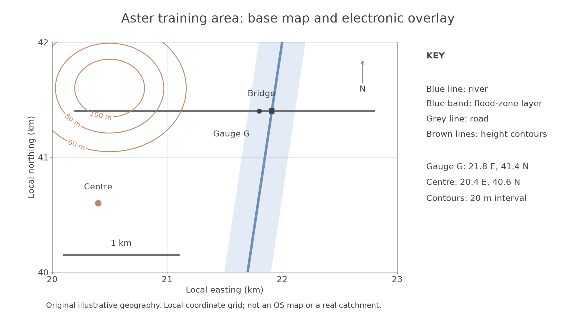
Original illustrative GIS layers. The blue band represents a modelled zone, not a measured flood or a real safety assessment.

The bridge crosses the river inside the band; the centre lies outside it. This supports a comparison of mapped exposure, but it cannot prove the bridge will flood in a particular event. Ask how the zone was modelled, its date and resolution, and which flood sizes or defences it includes. A point close to its edge may be sensitive to location error. Overlaying different coordinate systems without correct alignment can create a false spatial match.

Use GIS to map both primary and secondary evidence: record site coordinates, attach measurements, choose a meaningful symbol and show a key. A very large symbol must not conceal neighbouring sites. Save the layer names, dates, units and source information with the analysis so another person can reproduce the comparison.

Reading change in remote images

Remote sensing records the Earth's surface from aircraft or satellites. Compare the same extent, orientation and season where possible; a difference in shadow, tide or vegetation season can imitate change. Resolution limits the smallest feature that can be distinguished. A coloured pixel may contain several roofs, gardens and roads.

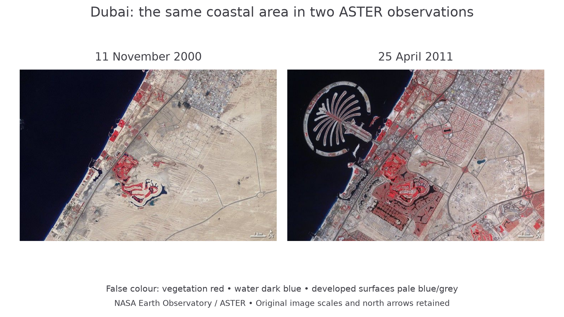
NASA Earth Observatory ASTER imagery: 11 November 2000 and 25 April 2011. These are false-colour observations: vegetation is red, water dark blue and developed surfaces mainly pale blue or grey. The original scale bars and north arrows are retained.

The later image shows a palm-shaped offshore development where the earlier image shows open water. Inland, many new road patterns and developed surfaces replace the more open desert area. These are observable changes. The images alone do not show household income, whether every building was occupied, or whether residents considered the change beneficial. Those questions need additional evidence. Image date is the observation date, not the date on which a webpage was updated.

Researching census evidence

A census records characteristics of a population at a reference time. The ONS Census maps tool, for example, displays England and Wales data referring to Census 2021. A map published or accessed later still describes that reference population. Choose the relevant topic and geographic area, inspect the variable's definition and denominator, and download or record the data with its source and date.

Suppose two neighbourhoods each contain 200 households using a particular heating fuel. One has 400 households and the other 2000. Their shares are 50% and 10%; equal counts conceal a very different local pattern. Boundary changes, non-response, classification changes and population change can complicate comparisons between censuses. An area's average is not a description of every resident.

Combine a census layer with field observations only when the places and concepts correspond. A survey of shoppers on one Saturday is not a census of residents. It may still provide a useful contrasting perspective if its different population is stated. Keep a copy of the actual figures used: an assessment should not depend on a live tool displaying the same screen months later.