Appendix 4, Appendix 6 - Choosing and constructing data displays

From observations to a useful table

Raw observations need an organised record before a graph can be trusted. A tally chart groups occurrences into stated categories, often using groups of five tally marks to reduce counting errors. Convert the tallies into frequencies and check that their total equals the number of valid observations. Keep “missing”, “not observed” and a genuine zero distinct.

For an original simulated survey of 20 journeys, the counts are walk 8, cycle 4, bus 6 and car 2. The categories refer to each person's main mode for one journey, so each person is counted once. If people could select several modes, the total could exceed 20 and a pie chart of exclusive shares would be misleading.

Preserve the original records when processing them in a spreadsheet. Put units in headings, keep one observation per row, check for impossible values and use consistent category names. Sorting only one column would detach measurements from their sites. A frequency table summarises evidence; it should not erase the place, time and method needed to interpret it.

Bars, pies and pictograms

A bar chart compares categories. Put travel modes on the horizontal axis, frequency on the vertical axis, use equal-width bars and leave gaps. Start a length-based bar scale at zero so a bar twice as high represents twice the count. A divided or compound bar separates each total into components. Stacking two sites' modes can compare composition, but only the bottom category shares a baseline; exact comparison of upper components may be harder.

A pie chart shows parts of a complete whole. Calculate each sector angle as share × 360°. For the 20 journeys, walking is 40% and occupies 144°; cycling 20% occupies 72°; bus 30% occupies 108°; car 10% occupies 36°. Check the angles sum to 360°. Use a key and state the sample total. Two pies with equal-looking sectors can hide very different sample sizes.

A pictogram uses a repeated symbol with a numerical key. If one symbol represents four journeys, eight walkers need two symbols, six bus journeys need one and a half, and two car journeys need half. Keep symbol size constant: doubling both width and height quadruples its area and can exaggerate the count.

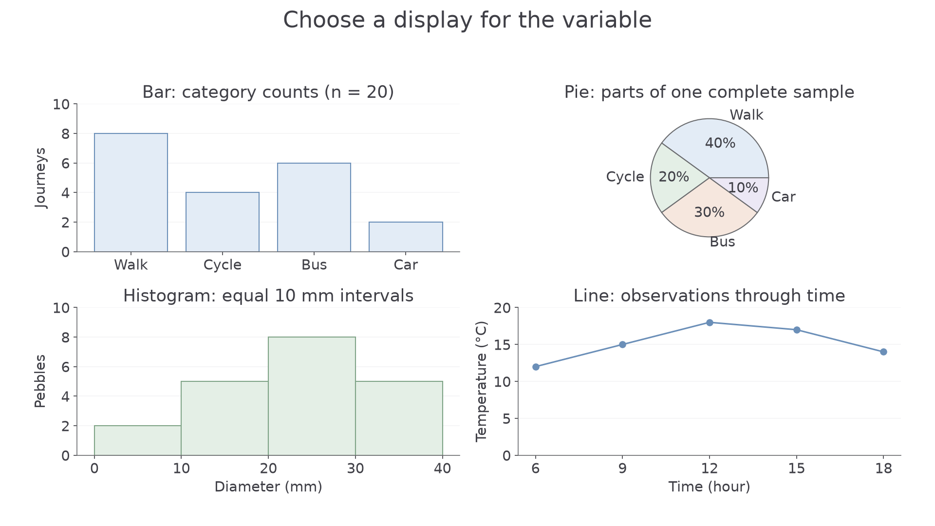
Original simulated training data. Each panel uses the representation suited to its variable; the histogram intervals are all 10 mm wide.

Lines and continuous intervals

A line graph shows change along an ordered, continuous axis such as time or distance. Choose a regular scale, plot each paired observation and join successive points when that connection is meaningful. A temperature measurement at 09:00 and another at 12:00 do not reveal every fluctuation between them; the connecting line summarises the change. Unequal time gaps must occupy unequal distances on the axis.

A histogram groups a continuous variable into class intervals. In the figure, sediment diameter is grouped into 0–<10, 10–<20, 20–<30 and 30–<40 mm, with frequencies 2, 5, 8 and 5. Each boundary belongs to one class only: a 20 mm pebble enters 20–<30. The bars touch because the measurement scale is continuous. With these equal class widths, frequency can be used as the height; the tallest bar identifies the modal class, 20–<30 mm. Unequal intervals require a different height calculation, so do not compare their raw heights as frequencies without checking the axis.

Construction needs a title, labelled axes and units, correct scales, accurate plotting and a clear key for several series. On paper, choose scales that use the available space and can be subdivided reliably. In digital software, check automatically chosen scales rather than accepting an exaggerated pattern. Draw a small graph yourself to test the method; when submitting a drawing, use the available drawing or image-upload response so the representation itself can be checked.

Paired data and qualitative evidence

A scatter graph plots two measurements for the same observation: for example, distance downstream and velocity at each site. Put the explanatory variable on the horizontal axis where appropriate, label both units and plot one point per pair. Do not join the dots in recording order. A line of best fit summarises a relationship rather than connecting every local fluctuation; its interpretation is developed in the statistics lesson.

Qualitative evidence such as interviews and photographs needs a presentation method that retains meaning. A short, accurately attributed quotation can explain why an EQS score matters to a resident; an annotated photograph can locate the physical evidence behind it. Group interview material into transparent themes, but retain contrasting or unusual views. A word cloud shows word frequency, not agreement, importance or the reasons behind a statement; “not safe” can become misleading if “not” is removed.

Choose displays by the enquiry. A located pie chart can compare journey-mode shares between sites, while a scatter graph can test whether those shares vary with distance from a station. One makes composition visible; the other makes a relationship visible. Neither automatically explains the cause. In a fieldwork conclusion, use both primary and secondary evidence and explain why each display supports the comparison you make.