1.3 - Tables, graphs and scatter diagrams
Learn to organise frequencies, construct suitable data displays and read their patterns without confusing categories, continuous measurements and paired observations.
Organising frequencies and tallies
A frequency is the number of observations belonging to a value, category or class interval.
Consider this original illustrative sequence of study-setting preferences: Q, M, Q, E, Q, M, Q, Q, M, Q, Q, M, Q, E, Q, M, Q, Q, M, Q. Here Q means quiet, M music and E either. Enter each response once, adding one tally to its category. Grouping tally marks in fives makes counting easier; the fifth mark crosses the preceding four when handwritten.
| Setting | Tally groups shown as counts | Frequency |
|---|---|---|
| Quiet | 5 + 5 + 2 | 12 |
| Music | 5 + 1 | 6 |
| Either | 2 | 2 |
| Total | 20 |
Give columns informative headings and check that the frequencies add to the original number of responses. A tally is a recording aid; the frequency column is the numerical summary. For measurement intervals, define non-overlapping boundaries before tallying. “10 to under 20 seconds” puts a time of 20 in the next interval, preventing double counting. The table preserves counts but grouping loses the exact values within each interval.
Constructing bar and pie charts
Bar and pie charts display category frequencies in different ways.
A bar chart has separate equal-width bars with gaps because the categories are distinct. For the preference table, label the horizontal axis “Preferred setting” and the vertical axis “Number of responses”. Choose an even scale, such as 0 to 14 in steps of 2, starting at zero to avoid exaggerating relative bar heights. Draw bars reaching 12, 6 and 2; a clear title tells the reader what responses are represented. A bar chart can also compare means for separate experimental conditions, with the vertical axis labelled for the mean and its units rather than frequency.
A pie chart represents parts of one whole. Convert each frequency into a fraction of 20, then multiply by a full circle's 360 degrees:
Quiet has and angle 216°; music has 30% and 108°; either has 10% and 36°. The angles total 360°. Draw a circle, measure consecutive sectors using a protractor, and label categories or provide a clear key. Do not draw slices directly from raw counts as degree values. A pie chart shows relative shares clearly, but small differences between categories may be easier to compare using bar heights.
[DIAGRAM: asset_slug: rm15_bar_pie; file: rm15_bar_pie.png; description: Bar and pie charts of original illustrative setting frequencies 12 quiet, 6 music and 2 either, with sectors 216, 108 and 36 degrees]
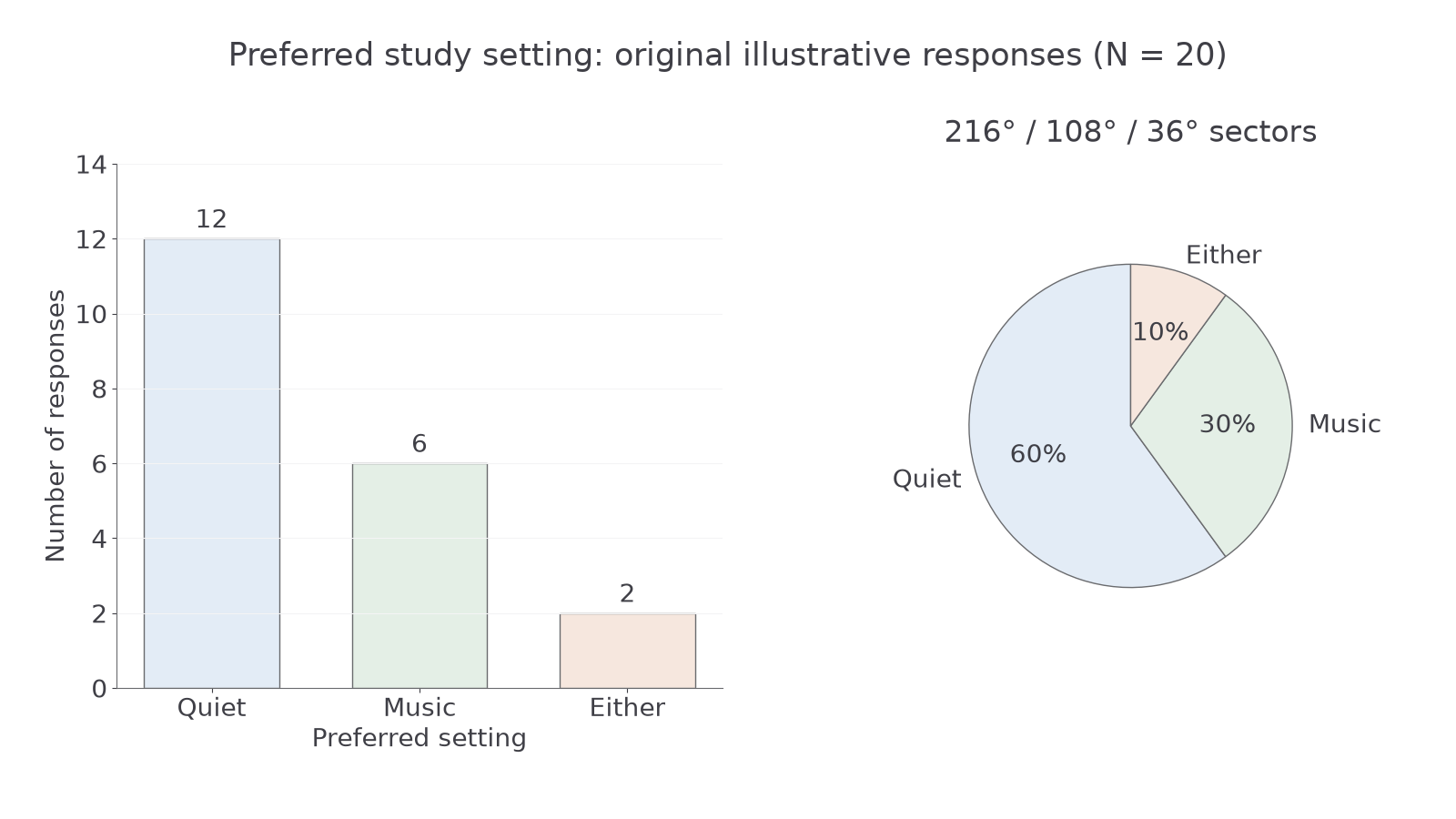
Diagram description: The same 20 original illustrative responses appear as separate bars and as shares of a circle.
For notebook practice, construct both displays for a different original illustrative dataset: visual summaries 8, written summaries 5 and spoken summaries 7, total 20. Check bar heights against counts and pie sectors against a complete circle.
Constructing a histogram
A histogram represents the distribution of a numerical variable grouped into continuous class intervals.
Original illustrative completion times have frequencies 2, 5, 8, 4 and 1 in the intervals 0 to under 10, 10 to under 20, 20 to under 30, 30 to under 40 and 40 to under 50 seconds. To construct the histogram, mark boundaries 0, 10, 20, 30, 40 and 50 on the time axis, use an equal frequency scale, and draw a rectangle over each entire interval. The rectangles touch because the intervals meet. They represent 20 participants, with the modal class 20 to under 30 seconds.
[DIAGRAM: asset_slug: rm15_histogram; file: rm15_histogram.png; description: Histogram of five equal ten-second completion-time classes with frequencies 2, 5, 8, 4 and 1]
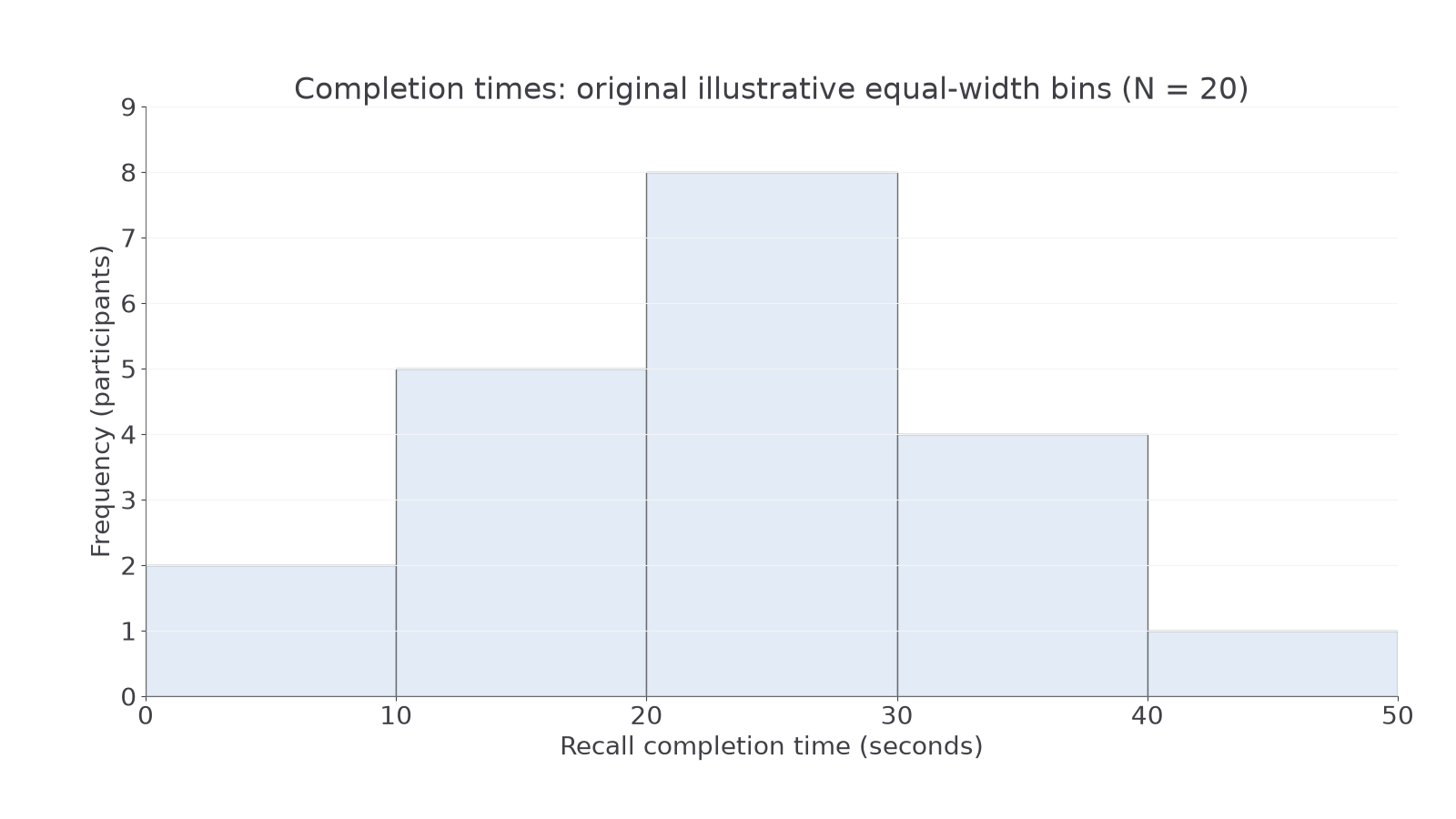
Diagram description: Touching bars cover the whole continuous time scale, with the tallest bar at 20 to under 30 seconds.
With equal-width bins, heights can show frequencies directly. If widths differ, use frequency density, frequency divided by class width, so rectangle area rather than height represents frequency. Otherwise a wide interval can misleadingly appear more frequent. Do not use gaps merely because few observations occur: a zero-frequency interval retains its place on the axis.
From a grouped histogram we can identify the modal class and broad shape, but not every exact time or an exact mean without additional information. For notebook practice, plot original illustrative frequencies 1, 4, 6 and 3 in equal intervals 0 to under 5, 5 to under 10, 10 to under 15 and 15 to under 20 seconds. Label the boundaries and total the frequencies before drawing.
Plotting change with a line graph
A line graph shows how a numerical quantity changes across a meaningful ordered sequence such as time or practice trials.
For original illustrative practice trials 1, 2, 3 and 4, mean response times are , , and milliseconds. Convert these to 420, 390, 370 and 365 ms before plotting. Put trial number on the horizontal axis, mean response time with its units on the vertical axis, and select equal intervals on each axis. Plot (1, 420), (2, 390), (3, 370) and (4, 365), then join successive observations in order.
[DIAGRAM: asset_slug: rm15_line; file: rm15_line.png; description: Line graph of original illustrative mean response times decreasing from 420 to 365 milliseconds over four practice trials]
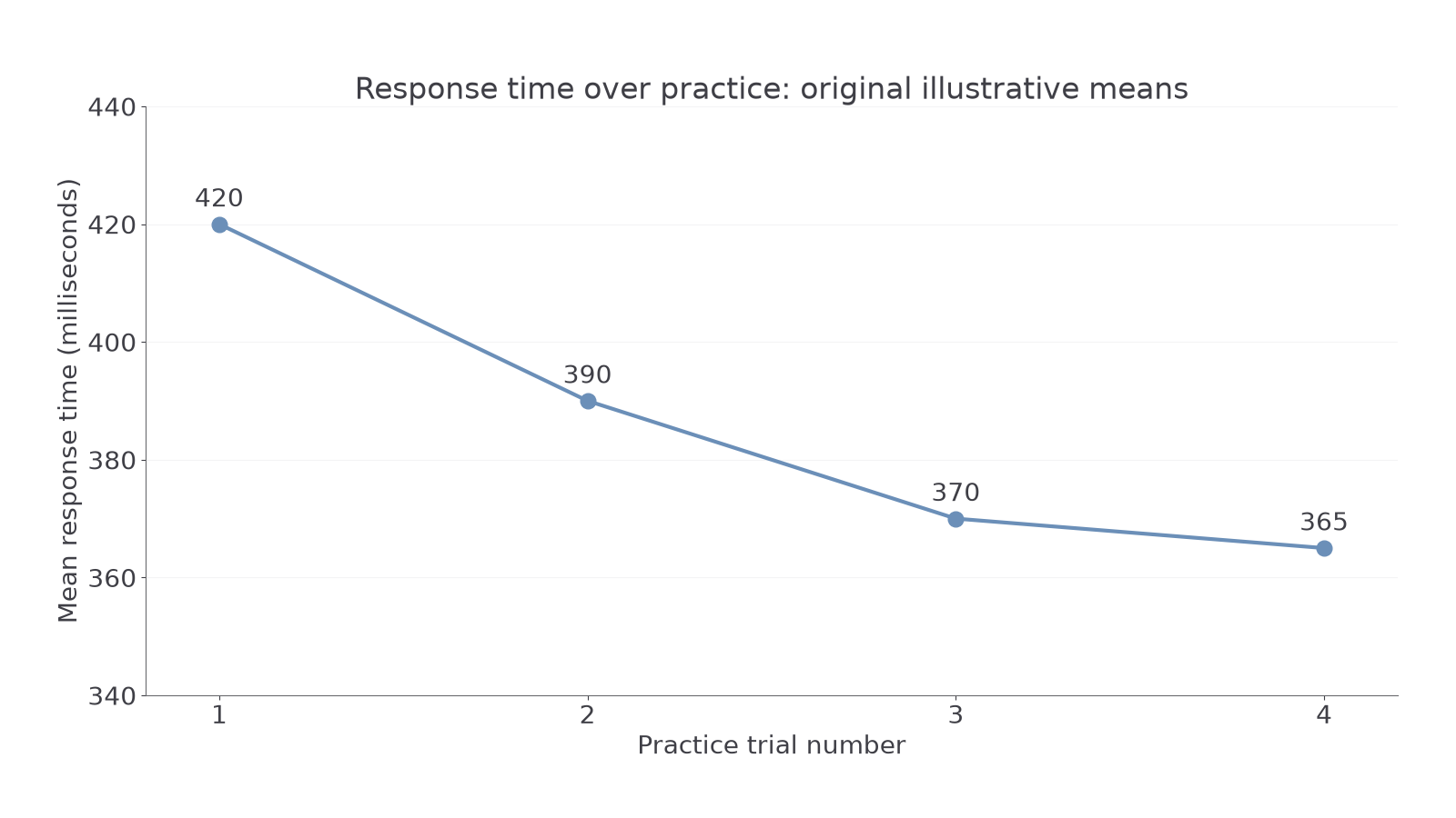
Diagram description: Response times fall most between trials 1 and 2 and then decrease more slowly.
The vertical scale shown starts at 340 ms, making small changes visible; read the labelled scale rather than treating the height above the page's bottom as the magnitude. Clearly disclose any shortened scale. The decrease is 55 ms overall, and the first change of 30 ms is greater than the last change of 5 ms. Connecting points represents progression across trials, not measured results at every point along each segment. Do not connect unordered categories such as quiet, music and either with a line.
For notebook practice, plot means of 15, 12, 10 and 9 errors for sessions 1–4. Use a title, labelled equal scales and consecutive joins, then identify where the greatest decrease occurs.
Plotting pairs and interpreting correlation
A scatter diagram keeps two measurements from the same person together as one point.
Six original illustrative participants have revision hours and words recalled as pairs (1, 4), (2, 6), (3, 5), (4, 9), (5, 8) and (6, 11). Label revision time in hours on the horizontal axis and words recalled out of 12 on the vertical axis. Choose equal scales, locate each horizontal value, then move to its paired vertical value and mark one dot. Plot all six pairs exactly. Do not sort one variable independently of the other or join participants' dots in order.
[DIAGRAM: asset_slug: rm15_scatter; file: rm15_scatter.png; description: Scatter diagram of six original illustrative revision-hour and recall pairs showing an imperfect positive association]
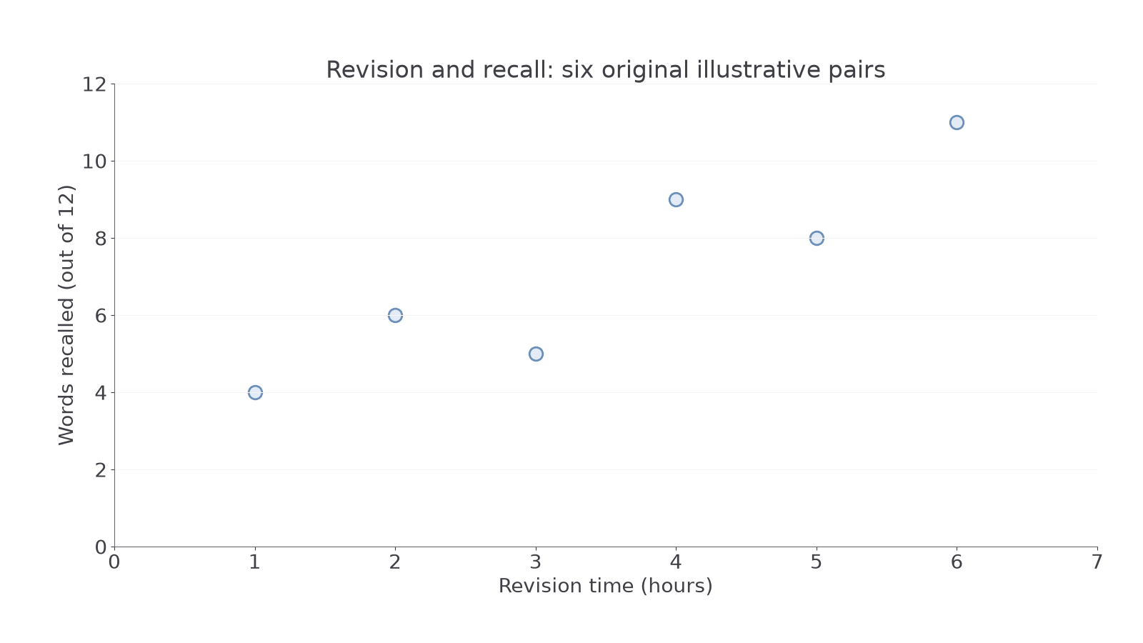
Diagram description: Higher revision hours generally accompany more words recalled, with deviations from a perfect straight pattern.
An upward tendency is a positive correlation; a downward tendency is negative. A scattered cloud without a clear increasing or decreasing tendency suggests no clear linear or monotonic correlation. A strong pattern has points closer to its trend, while an imperfect correlation allows exceptions. The displayed positive association does not prove that revision caused recall to improve: motivation might influence both, and the sample is small. A correlation coefficient or significance decision requires further analysis.
For notebook practice, plot original illustrative sleep-hour and error-count pairs (4, 9), (5, 8), (6, 6), (7, 7), (8, 3). Keep the pairs intact, then describe the direction with a cautious conclusion. A spreadsheet can help construct each display, but verify its graph type, data range, labels and scales yourself.