1.3 - Distributions, significance and errors
Learn how distributions describe scores and how probability, significance thresholds and decision errors limit conclusions from research.
Normal and skewed distributions
A distribution describes where scores are concentrated and how they extend across a scale.
A normal distribution is a symmetric, single-peaked bell-shaped distribution. Most observations lie near its centre, and progressively fewer lie far away in either direction. In the ideal normal distribution, mean, median and mode coincide. The mean locates the centre and SD describes spread: a greater SD gives a wider, flatter curve when the total probability remains the same. A real small sample need not form a perfect bell even when its population is approximately normal.
A positive skew has a long tail towards higher values; many observations are lower and a few are unusually high. For example, an easy task might produce mostly short completion times and a few long ones. A negative skew has a long tail towards lower values; an easy test with a maximum score might produce mostly high scores and a few low ones. Name the skew from its tail, not the location of the peak.
In the conventional single-peaked shapes below, positive skew places the mean to the right of the median and mode, while negative skew places it to their left. Extreme values pull the mean towards the tail. The median may better represent a typical score when the data are skewed. The familiar ordering is a guide to these shapes, not a theorem about every irregular or multi-peaked dataset.
[DIAGRAM: asset_slug: rm16_distributions; file: rm16_distributions.png; description: Original theoretical normal, positive-skew and negative-skew density curves with labelled mean, median and mode]
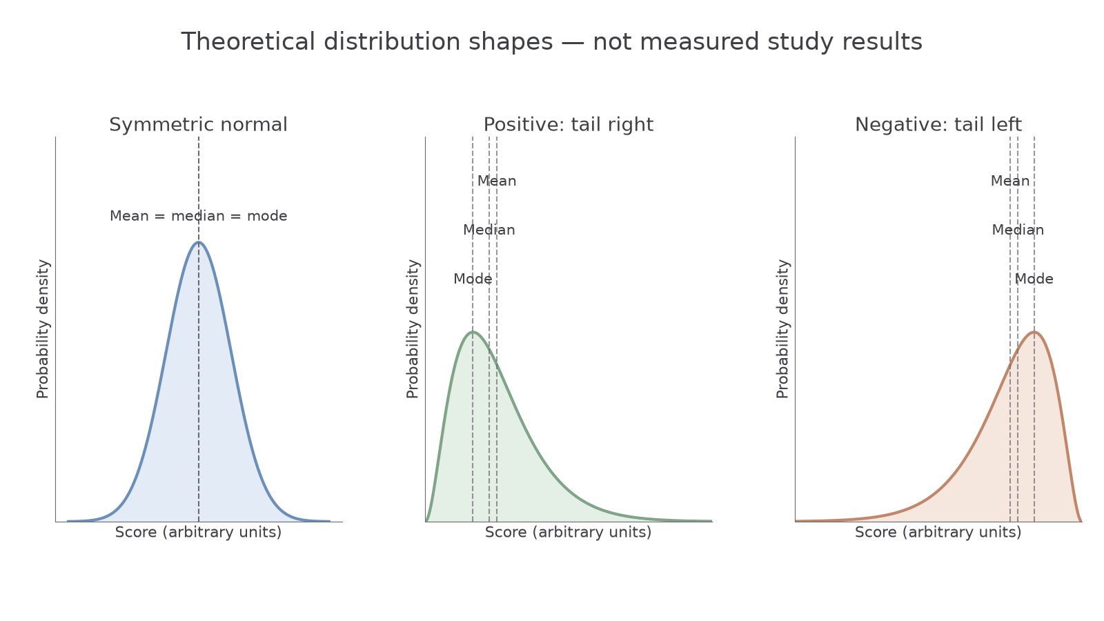
Diagram description: The normal curve is symmetric; the skewed curves have opposite tail directions and means pulled towards their tails. These are theoretical illustrations, not research results.
Understanding simple probability
Probability measures how likely an event is on a scale from 0 to 1.
Zero means impossible under the stated model and one means certain. For equally likely outcomes, divide the number of favourable outcomes by the total number of possible outcomes. A fair six-sided die has probability of showing six, or about 0.167. Two favourable faces out of six give , about 33.3%. Equal likelihood is an assumption: the same calculation is not automatically valid for an unfair die.
In an original illustrative dataset, 12 of 40 participants report using flashcards. Selecting one recorded participant uniformly at random gives probability that they reported flashcards. This is 30%, not a 30% probability that flashcards are effective. It describes this selection from these records, not necessarily the whole student population.
Independent events multiply: two heads in two independent fair coin tosses have probability . However, one participant's two responses may be related; do not assume independence simply because there are two observations. Probabilities require a stated event and conditions, not an unexplained percentage.
Significance levels and the null hypothesis
Inferential analysis asks whether the observed pattern would be sufficiently unusual under a null model to reject it.
The null hypothesis usually states no population difference or association of the kind being investigated. A p-value is the probability, assuming the null model and test assumptions, of a result at least as extreme as the observed result. It is not the probability that the null hypothesis is true or the percentage of the result “caused by chance”.
The researcher chooses a significance level, usually denoted , before examining the outcome. At , the decision threshold is 5%; at , it is 1%, requiring stronger evidence against the null model. Under the usual inclusive rule, reject the null when ; a task stating a strict inequality should be interpreted exactly as supplied.
For an original illustrative test of a difference in recall between two conditions, is significant at 0.05 but not at 0.01. Reject the null at the preselected 0.05 level. If instead , fail to reject it at 0.05: the evidence is insufficient, rather than proof that the groups are identical. Always state the conclusion in terms of the actual research question.
Significance does not establish a large or useful effect, causation, valid measurement or representative sampling. A small difference can be significant in a large sample, and an important difference may be undetected in a small noisy sample. Evaluate the design and the descriptive results alongside the statistical decision.
Type I and Type II errors
A statistical decision can be wrong because the true population situation is not directly known.
| Actual population situation | Reject the null | Fail to reject the null |
|---|---|---|
| Null is true | Type I error | Correct decision |
| Null is false | Correct decision | Type II error |
A Type I error, or false positive, rejects a true null hypothesis. A researcher may conclude that a memory aid changes recall when the population difference is actually absent. A Type II error, or false negative, fails to reject a false null hypothesis: a real population difference is missed.
At a correctly calibrated 0.05 threshold, the long-run Type I error probability is at most 5% when the null model and assumptions hold. This does not mean a particular significant conclusion has a 5% probability of being wrong. Reducing the threshold to 0.01 lowers false-positive risk but, other things equal, can increase Type II risk because fewer results qualify for rejection. The two error probabilities are not 5% and 95% complements.
The chance of detecting a real effect is power, equal to one minus the Type II error probability. A larger appropriate sample and a less noisy valid measurement can improve detection, but do not cure systematic bias. Select a threshold and design in advance: choosing a threshold only after seeing the p-value undermines the intended error control.